aoa4dl – Area of Applicability for Deep Learning: Exploring Latent Space Geometry of Earth Observation Models

Research question

Area of Applicability (Meyer and Pebesma 2021) defines the domain in which a model is trusted to operate within estimated performance measures

Our hypothesis is that:

Latent representations learned by deep models provide a computationally efficient and reliable basis for defining an Area of Applicability for Earth Observation models.

We are analyzing the question:

Under which conditions do distance-based confidence scores in the latent space of a deep model favourably delinate the Area of Applicability?

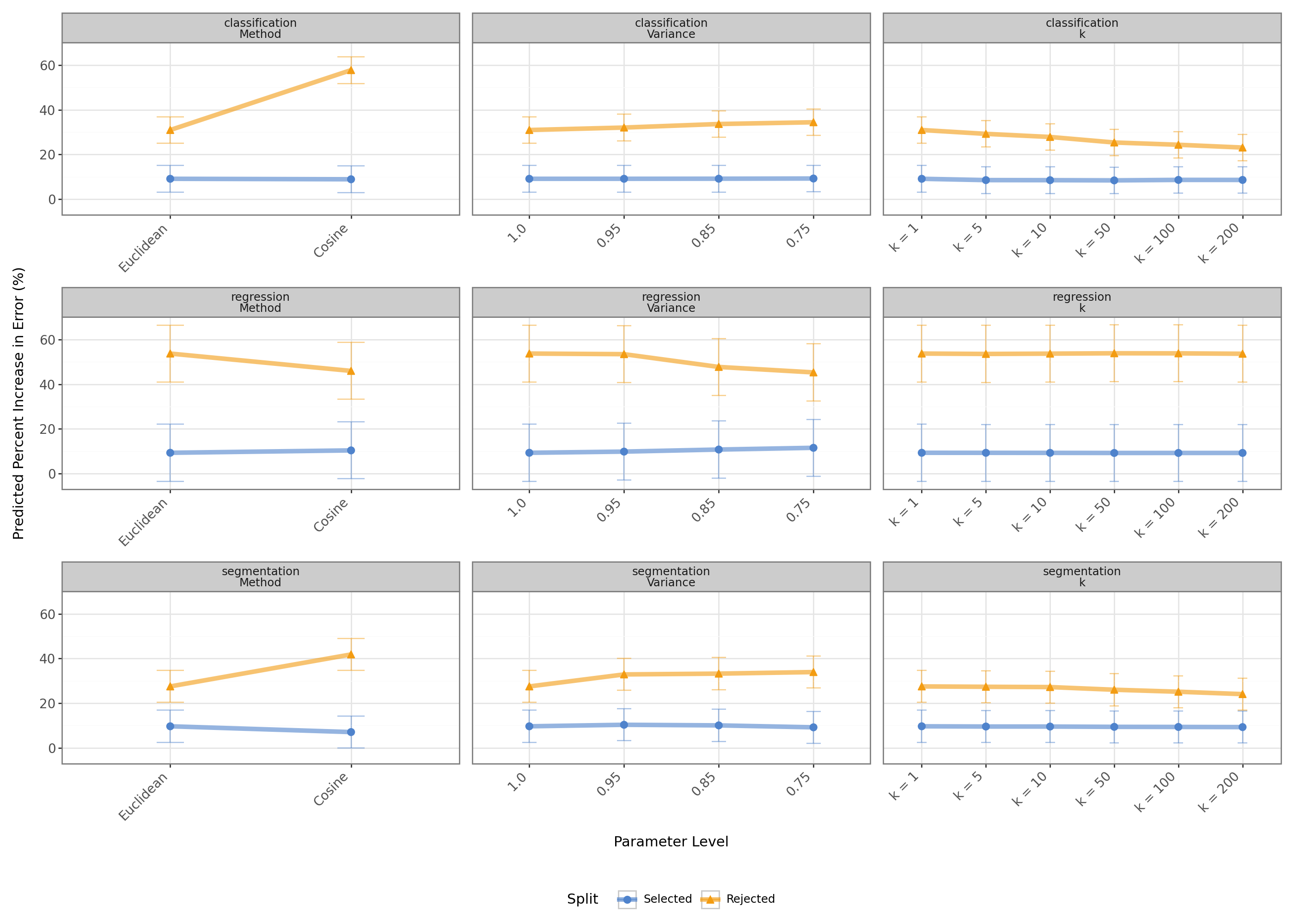
Average effects of analysed parameters on preservation and separation for classification.

Distances in representation space

Distances between training points and calibration (blue) and test (orange) sample.

Errors inside (blue) and outside (orange) the area of applicability versus reference error.

Problem setting

In the real world, models might be used for inference on samples which are outside of their domain of application.

Example of overconfident predictions for OOD samples (Hou 2023.)

Neural network-based classifiers may silently fail when the test data distribution differs from the training data. For critical tasks such as medical diagnosis or autonomous driving, it is thus essential to detect incorrect predictions based on an indication of whether the classifier is likely to fail.
Jaeger et al. (2023)

Problem setting

We are aiming to define a Selective Inference Model for deep learning models in Earth Observation:

\[ h(x) = \begin{cases} \varnothing, \; \text{if} \; g(x) = 1, \\ f(x), \; \text{if} \; g(x) = 0. \end{cases} \tag{1}\]

We evaluate the candidates based on two criteria:

Preservation: accepted inputs should approximately preserve the model’s estimated performance
Separation: rejected inputs should have significantly higher error than accepted ones

Dataset

We use the refined BigEarthNet (reBEN) dataset (Clasen et al. 2025), which is a large-scale benchmark for remote sensing image analysis
It consists of 480,038 Sentinel-2 image patches from 10 European countries, covering 125 tiles
Each image patch comes with a pixel-wise land cover classification based on the CORINE Land Cover dataset
This allows to construct and analyze three different tasks:
- C: image-level multi-label classification
- R: image-level multi-target regression
- S: pixel-level segmentation

Dataset

Number of images and tiles in the refined BigEarthNet (v2) dataset.
Country	Train	Validation	Test	Total	Tiles
Austria	24,972	10,649	8,176	43,797	16
Belgium	7,837	3,217	142	11,196	6
Finland	74,293	40,132	40,802	155,227	44
Ireland	22,482	12,687	13,157	48,326	9
Kosovo	849	487	280	1,616	1
Lithuania	23,170	12,128	13,067	48,365	15
Luxembourg	1,888	1,131	441	3,460	4
Portugal	43,721	22,862	23,209	89,792	12
Serbia	36,967	17,906	18,512	73,385	17
Switzerland	1,692	1,143	2,039	4,874	1
Total	237,871	122,342	119,825	480,038	125

Methodology

Linear mixed effects model

\[ Y_i = X_i^\top \beta + b_{c(i)} + \varepsilon_i \tag{2}\]

with:

\(Y_i\) being the increase in error for subset \(i\),
\(X_i\) being the vector of fixed effects (rejected vs. selected, method, variance, K),
\(\beta\) being the vector of fixed effect coefficients,
\(b_{c(i)}\) being the random intercept for country \(c(i)\),
and \(\varepsilon_i\) being the residual error.

Results

Percentage of rejected samples

Average rejected percentage for classification (C) by country and distance metric. Error bars represent the range over all configurations.

Increase in error

Average increase in error for classification (C) by country and selection. Error bars represent the range over all configurations.

Selected and rejected samples

Coefficients

Parameter	Coef.	Std.Err.	\(P>\|z\|\)	Sig.
Intercept (Euclidean, Selected)	9.123	3.032	0.0026	**
Rejected	21.839	1.034	0	***
Method: Cosine	-0.213	0.463	0.6454
Variance: 0.95	0.007	0.654	0.9913
Variance: 0.85	0.041	0.654	0.9496
Variance: 0.75	0.128	0.654	0.8443
\(k = 5\)	-0.589	0.801	0.462
\(k = 10\)	-0.62	0.801	0.4391
\(k = 50\)	-0.711	0.801	0.3752
\(k = 100\)	-0.496	0.801	0.5358
\(k = 200\)	-0.512	0.801	0.5225
Rejected x Method: Cosine	27.024	0.654	0	***
Rejected x Variance: 0.95	1.088	0.925	0.2396
Rejected x Variance: 0.85	2.644	0.925	0.0043	**
Rejected x Variance: 0.75	3.343	0.925	0.0003	***
Rejected x \(k = 5\)	-1.137	1.133	0.3155
Rejected x \(k = 10\)	-2.493	1.133	0.0278	*
Rejected x \(k = 50\)	-4.877	1.133	0	***
Rejected x \(k = 100\)	-6.109	1.133	0	***
Rejected x \(k = 200\)	-7.342	1.133	0	***

Table 1: Results of the linear mixed effects model for the classification task. Reference categories: Split = Selected (error of accepted samples), Method = Euclidean, Variance = 1.0, \(k\) = 1. Significance: \(^*\) \(p < 0.05\), \(^{**}\) \(p < 0.01\), \(^{***}\) \(p < 0.001\).

Effects

Change in error depending on changes in contrasts by analysed parameter, and selection result.

Discussion

Investigating the Area of Applicability for deep learning models in Earth observation is crucial for ensuring reliable and trustworthy model performance in real-world applications
Compared to the classical OOD detection setting, the AOA framework emphasizes the importance of defining a domain of application for a model based on estimated performance measures, rather than just detecting OOD samples
KNN-based confidence scores in the latent space of a deep model correlate with model performance, with a considerable effect size that depends on the task and the choice of distance function
the choice of distance function and its parameters moderately effect the results, but there is no clear pattern across tasks
further research is needed to explore if these findings translate to other datasets and tasks

References

Clasen, Kai Norman, Leonard Hackel, Tom Burgert, Gencer Sumbul, Begüm Demir, and Volker Markl. 2025. “reBEN: Refined BigEarthNet Dataset for Remote Sensing Image Analysis.” arXiv. https://doi.org/10.48550/arXiv.2407.03653.

Feranec, Jan, Tomas Soukup, Gerard Hazeu, and Gabriel Jaffrain, eds. 2016. European Landscape Dynamics: CORINE Land Cover Data. Boca Raton: CRC Press. https://doi.org/10.1201/9781315372860.

Gawlikowski, Jakob, Sudipan Saha, Anna Kruspe, and Xiao Xiang Zhu. 2021. “Out-of-Distribution Detection in Satellite Image Classification.” arXiv. https://doi.org/10.48550/arXiv.2104.05442.

Guo, Chuan, Geoff Pleiss, Yu Sun, and Kilian Q. Weinberger. 2017. “On Calibration of Modern Neural Networks.” arXiv. https://doi.org/10.48550/arXiv.1706.04599.

Hendrycks, Dan, and Kevin Gimpel. 2018. “A Baseline for Detecting Misclassified and Out-of-Distribution Examples in Neural Networks.” arXiv. https://doi.org/10.48550/arXiv.1610.02136.

Jaeger, Paul F, Carsten Tim Lüth, Lukas Klein, and Till J. Bungert. 2023. “A Call to Reflect on Evaluation Practices for Failure Detection in Image Classification.” In International Conference on Learning Representations. https://openreview.net/forum?id=YnkGMIh0gvX.

Malkov, Yu A., and D. A. Yashunin. 2020. “Efficient and Robust Approximate Nearest Neighbor Search Using Hierarchical Navigable Small World Graphs.” IEEE Trans. Pattern Anal. Mach. Intell. 42 (4): 824–36. https://doi.org/10.1109/TPAMI.2018.2889473.

Meyer, Hanna, and Edzer Pebesma. 2021. “Predicting into Unknown Space? Estimating the Area of Applicability of Spatial Prediction Models.” Methods in Ecology and Evolution 12 (9): 1620–33. https://doi.org/https://doi.org/10.1111/2041-210X.13650.

Stewart, Adam J., Caleb Robinson, Isaac A. Corley, Anthony Ortiz, Juan M. Lavista Ferres, and Arindam Banerjee. 2025. “TorchGeo: Deep Learning With Geospatial Data.” ACM Trans. Spatial Algorithms Syst. 11 (4): 15:1–28. https://doi.org/10.1145/3707459.

Sun, Yiyou, Yifei Ming, Xiaojin Zhu, and Yixuan Li. 2022. “Out-of-Distribution Detection with Deep Nearest Neighbors.” In Proceedings of the 39th International Conference on Machine Learning, 20827–40. PMLR. https://proceedings.mlr.press/v162/sun22d.html.

Backup slides

Formalisation

Given a trained model \(f: \mathcal X \mapsto \mathcal Y\) and a novelty score function \(s: \mathbb{R^d} \mapsto \mathbb{R^1}\).

We induce a decision function \(g\):

\[ g_{\lambda}(x|s) = \mathbb{1}{ \{ s(x) > \lambda \} }. \tag{3}\]

Traditionally, we evaluate if \(g\) is successful in detecting samples from another distribution (OOD detection): \[ g(x) = \begin{cases} OOD, \; \text{if} \; g(x) = 1, \\ ID, \; \text{if} \; g(x) = 0, \end{cases} \tag{4}\]

However, in many real-world applications, we are interested in accepting samples were the model is expected to perform well and rejecting those where it is expected to perform poorly:

\[ h(x) = \begin{cases} \varnothing, \; \text{if} \; g(x) = 1, \\ f(x), \; \text{if} \; g(x) = 0. \end{cases} \tag{5}\]

Linear mixed effects model

\[ \begin{aligned} Y_i &= \beta_0 + \beta_1\,\text{Rejected}_i + \beta_2\,\text{Method}_i + \beta_3\,\text{Variance}_i \\ &\quad + \beta_4\,K_i + \beta_5\,(\text{Rejected}_i \times \text{Method}_i) \\ &\quad + \beta_6\,(\text{Rejected}_i \times \text{Variance}_i) + \beta_7\,(\text{Rejected}_i \times K_i) + b_{c(i)} + \varepsilon_i \end{aligned} \]

Overall results

Change in increased error depending on changes in contrasts by task, parameter, and selection.

Preservation
- Selected samples ≈ +9% error; configs have no major effect
- Exception: lower PCA variance worsens R (+2.2% at 0.75)
Separation
- Rejected samples have much higher error (17–44%)
- Cosine: helps C (+27%) & S (+17%), hurts R (−8.9%)
- Lower PCA variance: helps C (+3.3%) & S (+6.9%), hurts R (−10.7%)
- Increasing K: no effect on R; harms C (-7.3%) and S (−3%)

Classification results

Average rejected percentage for classification (C) by country and distance metric. Error bars represent the range over all configurations.

Classification results

Average increase in error for classification (C) by country and selection. Error bars represent the range over all configurations.

Classification results

In-distribution error versus out-of-distribution error (each dot represents the average over a country dataset).

Classification results

Parameter	Coef.	Std.Err.	\(P>\|z\|\)	Sig.
Intercept (Euclidean, Selected)	9.123	3.032	0.0026	**
Rejected	21.839	1.034	0	***
Method: Cosine	-0.213	0.463	0.6454
Variance: 0.95	0.007	0.654	0.9913
Variance: 0.85	0.041	0.654	0.9496
Variance: 0.75	0.128	0.654	0.8443
\(k = 5\)	-0.589	0.801	0.462
\(k = 10\)	-0.62	0.801	0.4391
\(k = 50\)	-0.711	0.801	0.3752
\(k = 100\)	-0.496	0.801	0.5358
\(k = 200\)	-0.512	0.801	0.5225
Rejected x Method: Cosine	27.024	0.654	0	***
Rejected x Variance: 0.95	1.088	0.925	0.2396
Rejected x Variance: 0.85	2.644	0.925	0.0043	**
Rejected x Variance: 0.75	3.343	0.925	0.0003	***
Rejected x \(k = 5\)	-1.137	1.133	0.3155
Rejected x \(k = 10\)	-2.493	1.133	0.0278	*
Rejected x \(k = 50\)	-4.877	1.133	0	***
Rejected x \(k = 100\)	-6.109	1.133	0	***
Rejected x \(k = 200\)	-7.342	1.133	0	***

Table 2: Results of the linear mixed effects model for the classification task. Reference categories: Split = Selected (error of accepted samples), Method = Euclidean, Variance = 1.0, \(k\) = 1. Significance: \(^*\) \(p < 0.05\), \(^{**}\) \(p < 0.01\), \(^{***}\) \(p < 0.001\).

Regression results

Average rejected percentage for regression (R) by country and distance metric. Error bars represent the range over all configurations.

Regression results

Average increase in error for regression (R) by country and selection. Error bars represent the range over all configurations.

Regression results

In-distribution error versus out-of-distribution error (each dot represents the average over a country dataset).

Regression results

Parameter	Coef.	Std.Err.	\(P>\|z\|\)	Sig.
Intercept (Euclidean, Selected)	9.28	6.501	0.1534
Rejected	44.42	0.853	0	***
Method: Cosine	1.073	0.382	0.0049	**
Variance: 0.95	0.529	0.54	0.3273
Variance: 0.85	1.454	0.54	0.007	**
Variance: 0.75	2.229	0.54	0	***
\(k = 5\)	-0.013	0.661	0.9841
\(k = 10\)	-0.037	0.661	0.955
\(k = 50\)	-0.079	0.661	0.9043
\(k = 100\)	-0.075	0.661	0.9095
\(k = 200\)	-0.063	0.661	0.9239
Rejected x Method: Cosine	-8.836	0.54	0	***
Rejected x Variance: 0.95	-0.8	0.763	0.2943
Rejected x Variance: 0.85	-7.446	0.763	0	***
Rejected x Variance: 0.75	-10.667	0.763	0	***
Rejected x \(k = 5\)	-0.156	0.935	0.8672
Rejected x \(k = 10\)	-0	0.935	0.9998
Rejected x \(k = 50\)	0.205	0.935	0.8266
Rejected x \(k = 100\)	0.165	0.935	0.8602
Rejected x \(k = 200\)	-0.026	0.935	0.9781

Table 3: Results of the linear mixed effects model for the classification task. Reference categories: Split = Selected (error of accepted samples), Method = Euclidean, Variance = 1.0, \(k\) = 1. Significance: \(^*\) \(p < 0.05\), \(^{**}\) \(p < 0.01\), \(^{***}\) \(p < 0.001\).

Segmentation results

Average increase in error for segmentation (S) by country and selection. Error bars represent the range over all configurations.

Segmentation results

Average rejected percentage for segmentation (S) by country and distance metric. Error bars represent the range over all configurations.

Segmentation results

In-distribution error versus out-of-distribution error (each dot represents the average over a country dataset).

Segmentation results

Parameter	Coef.	Std.Err.	\(P>\|z\|\)	Sig.
Intercept (Euclidean, Selected)	9.657	3.651	0.0082	**
Rejected	17.845	0.836	0	***
Method: Cosine	-2.587	0.374	0	***
Variance: 0.95	0.67	0.529	0.2047
Variance: 0.85	0.406	0.529	0.4429
Variance: 0.75	-0.457	0.529	0.3867
\(k = 5\)	-0.104	0.647	0.8722
\(k = 10\)	-0.118	0.647	0.8559
\(k = 50\)	-0.247	0.647	0.7029
\(k = 100\)	-0.294	0.647	0.6502
\(k = 200\)	-0.361	0.647	0.5767
Rejected x Method: Cosine	16.905	0.529	0	***
Rejected x Variance: 0.95	4.702	0.747	0	***
Rejected x Variance: 0.85	5.324	0.747	0	***
Rejected x Variance: 0.75	6.887	0.747	0	***
Rejected x \(k = 5\)	-0.057	0.915	0.9505
Rejected x \(k = 10\)	-0.172	0.915	0.8506
Rejected x \(k = 50\)	-1.235	0.915	0.1774
Rejected x \(k = 100\)	-2.083	0.915	0.0229	*
Rejected x \(k = 200\)	-3.082	0.915	0.0008	***

Table 4: Results of the linear mixed effects model for the classification task. Reference categories: Split = Selected (error of accepted samples), Method = Euclidean, Variance = 1.0, \(k\) = 1. Significance: \(^*\) \(p < 0.05\), \(^{**}\) \(p < 0.01\), \(^{***}\) \(p < 0.001\).