Last updated: 2021-05-12
Checks: 7 0
Knit directory:
thesis/analysis/
This reproducible R Markdown analysis was created with workflowr (version 1.6.2). The Checks tab describes the reproducibility checks that were applied when the results were created. The Past versions tab lists the development history.
Great! Since the R Markdown file has been committed to the Git repository, you know the exact version of the code that produced these results.
Great job! The global environment was empty. Objects defined in the global environment can affect the analysis in your R Markdown file in unknown ways. For reproduciblity it’s best to always run the code in an empty environment.
The command set.seed(20210321) was run prior to running the code in the R Markdown file.
Setting a seed ensures that any results that rely on randomness,
e.g. subsampling or permutations, are reproducible.
Great job! Recording the operating system, R version, and package versions is critical for reproducibility.
Nice! There were no cached chunks for this analysis, so you can be confident that you successfully produced the results during this run.
Great job! Using relative paths to the files within your workflowr project makes it easier to run your code on other machines.
Great! You are using Git for version control. Tracking code development and connecting the code version to the results is critical for reproducibility.
The results in this page were generated with repository version 7fd4ff2. See the Past versions tab to see a history of the changes made to the R Markdown and HTML files.
Note that you need to be careful to ensure that all relevant files for the
analysis have been committed to Git prior to generating the results (you can
use wflow_publish or wflow_git_commit). workflowr only
checks the R Markdown file, but you know if there are other scripts or data
files that it depends on. Below is the status of the Git repository when the
results were generated:
Ignored files:
    Ignored:    .Rproj.user/
    Ignored:    data/DB/
    Ignored:    data/raster/
    Ignored:    data/raw/
    Ignored:    data/vector/
    Ignored:    docker_command.txt
    Ignored:    output/acc/
    Ignored:    output/bayes/
    Ignored:    output/ffs/
    Ignored:    output/models/
    Ignored:    output/plots/
    Ignored:    output/test-results/
    Ignored:    renv/library/
    Ignored:    renv/staging/
    Ignored:    report/presentation/

Untracked files:
    Untracked:  analysis/assets/
Note that any generated files, e.g. HTML, png, CSS, etc., are not included in this status report because it is ok for generated content to have uncommitted changes.
These are the previous versions of the repository in which changes were made
to the R Markdown (analysis/thesis-data.Rmd) and HTML (docs/thesis-data.html)
files. If you’ve configured a remote Git repository (see
?wflow_git_remote), click on the hyperlinks in the table below to
view the files as they were in that past version.
| File | Version | Author | Date | Message |
|---|---|---|---|---|
| Rmd | de8ce5a | Darius Görgen | 2021-04-05 | add content |
| html | de8ce5a | Darius Görgen | 2021-04-05 | add content |
1 Data
1.1 Area of Interest
To account for the hypothesis that aggregating predictor variables on the basis of watersheds will lead to higher detection accuracy compared to administrative boundaries, two different sets of spatial units are selected. The first represents sub-national administrative boundaries (referred to as adm hereafter) derived from the Natural Earth project in a vector format (South, 2017). Only polygons on the African continent as well as Madagascar from the third administrative level are selected. The procedure results in a total of 847 polygons covering the study area (Figure 1.1).
adm <- st_read("../data/vector/states_mask.gpkg", quiet = T)
adm <- st_make_valid(adm)
bas <- st_read("../data/vector/basins_simple.gpkg", quiet = T)
bas <- st_make_valid(bas)
crs <- st_crs("EPSG:3857")
adm <- st_transform(adm, crs)
adm <- st_simplify(adm, dTolerance = 1000, preserveTopology = T)
bas <- st_transform(bas, crs)
bas <- st_simplify(bas, dTolerance = 1000, preserveTopology = T)

tmap_options(max.categories = 50)

adm %<>%
  mutate(group_id = sov_a3) %>%
  dplyr::select(group_id)

plt1 = tm_shape(adm) +
  tm_polygons("group_id", border.col = "black", lwd = .2) +
  tm_legend(show = FALSE) +
  tm_layout(expression(paste(italic("adm"), " districts")),
            title.size = .8) +
  tm_scale_bar(position=c("left", "bottom"), width = .5)


bas_group = st_read("../data/raw/hydrosheds/hybas_03_simple.gpkg", quiet = TRUE)
bas_group %<>%
  st_transform(crs = crs) %>%
  mutate(group_id = as.factor(HYBAS_ID)) %>%
  dplyr::select(group_id) %>%
  st_simplify() %>%
  st_crop(bas)
adm$group_id = NULL
bas %<>%
  dplyr::select(geom)

plt2 = tm_shape(bas_group) +
  tm_polygons("group_id", lwd = 0, border.col = "white") +
  tm_shape(bas) +
  tm_borders("black", lwd = .2) +
  tm_legend(show = FALSE) +
  tm_layout(title = expression(paste(italic("bas"), " districts")),
            title.size = .8)

tmap_arrange(plt1, plt2)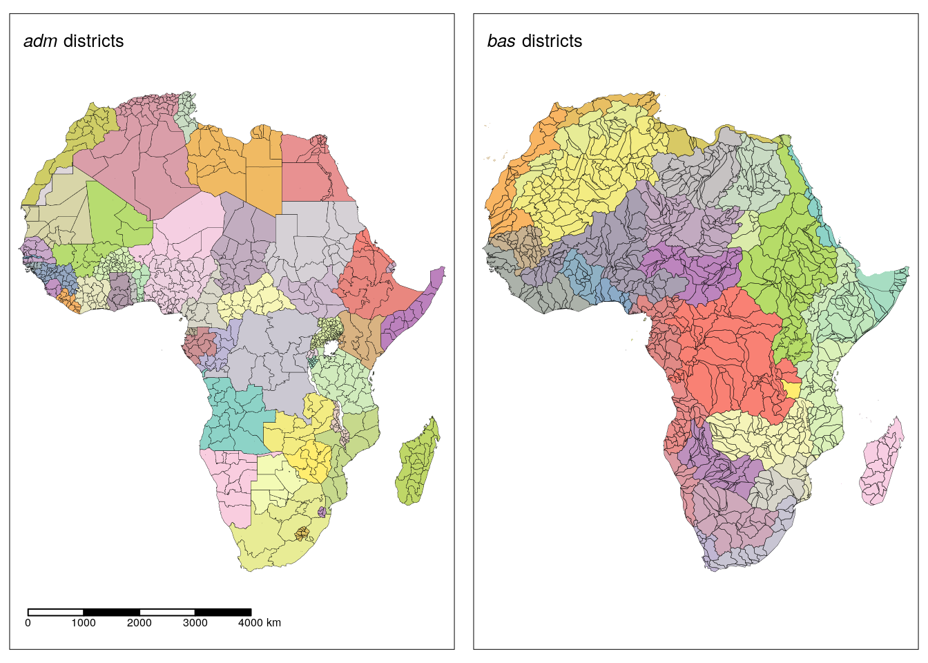
Figure 1.1: Overview of the administrative (left) and sub-basin districts (right) used for data aggregation.
| Version | Author | Date |
|---|---|---|
| de8ce5a | Darius Görgen | 2021-04-05 |
The second set of spatial units represents sub-basin watersheds (referred to as bas hereafter) which are downloaded from the HydroSHEDS project (Lehner et al., 2008). To keep the number of polygons comparable to the number of administrative units, the fifth level out of a total of 12 levels of watershed delineations is selected. The procedure results in a total number of 1013 polygons covering the African continent and Madagascar (Figure 1.1).
adm_area = st_area(adm) /  1e+6 # to km2
bas_area = st_area(bas) /  1e+6 # to km2

adm_sum = summary(adm_area)
bas_sum = summary(bas_area)

adm_sum = tibble(values = round(adm_sum, 3), col_names = names(adm_sum))
bas_sum = tibble(values = round(bas_sum, 3), col_names = names(bas_sum))

adm_sum["Spatial unit"] <- "*adm*"
bas_sum["Spatial unit"] <- "*bas*"

descr <- rbind(adm_sum, bas_sum)

descr %<>%
  pivot_wider(id_cols = "Spatial unit",
              values_from = values, names_from = col_names) %>%
  mutate(N = c(nrow(adm), nrow(bas))) %>%
  dplyr::select(c(names(.)[1], N, names(.)))
rm(bas, bas_group, adm)

descr %>%
  thesis_kable(escape = FALSE,
               caption = "Descriptive statistics on the area of the spatial aggregation units in km². (*adm* represents administrative units, *bas* represents sub-basin watersheds)",
               caption.short = "Descriptive statistics on the area of the spatial aggregation units.",
style = list(latex_options = c("HOLD_position")))| Spatial unit | N | Min. | 1st Qu. | Median | Mean | 3rd Qu. | Max. |
|---|---|---|---|---|---|---|---|
| adm | 847 | 3.697 | 3133.327 | 10881.78 | 39081.96 | 39393.61 | 734187.2 |
| bas | 1013 | 0.682 | 9298.121 | 21232.59 | 32614.09 | 43165.52 | 315931.1 |
The descriptive statistics of area distribution among the two different sets reveals that the sub-basin watersheds have a lower average value of 32,614.09 km² compared to 39,081.96 km², while the administrative units have the highest maximum value of 734,187.2 km² which is nearly twice as large as the largest watershed (Table 1.1).
Three different spatial buffers of 50, 100, and 200 km are processed for each district to include information on the geographical neighborhood. It is assumed that processes in the larger neighborhood of a district might influence the occurrence of conflicts. This influence can take the form of spillover effects for which empirical evidence has been found, e.g., for military spending (Phillips, 2015), reducing regional trade volumes (Murdoch and Sandler, 2004) or short-term reduction in economic growth (Murdoch and Sandler, 2002). These effects can manifest in environmental changes and reduction of agricultural production, as has been the case for Syria and Iraq during the war against the so-called Islamic State (Eklund et al., 2017). For Sub-Saharan Africa, additional evidence has been presented that spillover effects are more pronounced than in the rest of the world (Carmignani and Kler, 2016). For each of the buffered areas, the same variables are extracted as for individual districts, resulting in a 3-time increase in the data set size.
1.2 Spatiotemporal Aggregation
For the establishment of a regular data set used for the training process a number of predictor variables in the raster format need to be processed into a regular time series based on the spatial aggregation districts used for prediction (Table 1.3). Raw remote sensing scenes, as well as value-added raster products, vary greatly in the spatiotemporal resolution they are available at (Table 1.3). The resolution is a function of the technical prerequisites of a given sensor or statistical method in the case of socio-economic variables and design choices by the product providers. For example, together, both satellites equipped with the Moderate Resolution Imaging Spectroradiometer (MODIS) cover every point on earth every 1 to 2 days. However, certain products such as evaporation or gross primary productivity are processed to 8-day composites. This design choice was made to assure valid measurements of certain variables that might be blocked on some day, e.g., through persistent cloud coverage, especially in the tropics (Steven Running et al., 2017). Other products, such as precipitation data or population counts are available at a monthly or yearly temporal resolution, mainly due to the statistical processes involved in their production, e.g., in the latter case by relying on yearly survey data. To account for this variability in data set characteristics, the decision is made to aggregate on a monthly district level (district-months). A pixel-based approach, which would require the transformation of all data sets to a common spatial resolution, is rejected due to the very low occurrences of the response variables and the great variability of spatial resolutions across the data sets. That way, all data sets can be processed at or close to their native resolution since the final value for a given district-month is obtained by a zonal statistic operation. To this end, the R package gdalcubes was used (Appel and Pebesma, 2019). This package was specifically designed for the efficient harmonization of remote sensing products with varying spatiotemporal resolutions. It programmatically conducts the transformations needed to bring a given raster data set to the desired spatio-temporal resolution and provides efficient routines to calculate zonal statistics for the intersection areas between rasters and polygons.
For data sets that are available at a yearly time scale or static over the complete time-series a last-observation-carried-forward approach is0 chosen to obtain a monthly data set. For data sets that are available at a finer resolution, a suitable aggregation operation to the measured variable is chosen (Table 1.3). In summary, a vector data cube consisting of 847 (1013) districts for adm (bas) for 228 individual months (2001 to 2019) and 176 ((40 predictors + 4 responses) x 4 buffers) variables summing up to a total of 33,988,416 (40,649,664) individual data points is constructed. The individual variables selected for training are explained in detail in the following sections.
1.3 Response Variable
Data from UCDP is used for the response variable (Pettersson and Öberg, 2020). The data is an event database, meaning that every reported violent conflict with at least 25 fatalities per year is included as a single event. Each event is associated with information on involved actors, time, location, and estimated fatalities by party involved. Since the data is mainly collected automatically, inaccuracies concerning the exact location or the number of deaths are frequently observed. However, the information on the reliability for each logged event is included. The latest version of the database as of the time of writing this thesis for the African continent is used. Only events occurring between 2001 and 2019 are included. The data is further filtered to contain only events for which the quality of the geographic localization is assured to be accurate on the sub-national level. Also, only events are included with timestamps which are reported to be accurate on a monthly scale. The data is provided distinguishing between three different classes of conflict. These are state-based violence (referred to sb hereafter), non-state violence (ns), and one-sided violence (os) as defined in Gleditsch et al. (2002), Sundberg et al. (2012), and Eck and Hultman (2007), respectively. UCDP summarizes these definitions as “violence between two organized actors of which at least one is the government of a state, violence between actors of which neither party is the government of a state, and lastly, violence against unarmed civilians perpetrated by organized non-state groups or governments” (Allansson, 2021). For each class, a spatiotemporal aggregation based on the different analysis units on a monthly time scale is applied. Additionally, by a summation of casulties a fourth class representing a combination of the three base classes is introduced (referred to as cb). These aggregations represent the basic unit of analysis for this project and are used as the response objects for the detection algorithm. Because the final prediction problem is conceptualized as a binary classification task (peace vs. conflict) any district-month with fatalities greater than 0 is transformed to a value of 1, representing conflict, while district-months with no fatalities are assigned a value of 0, representing peace.
response_cube = readRDS("../data/vector/response_cube.rds")

response_cube %>%
  as_tibble() %>%
  filter(!(unit == "states" & id > 847),
         type %in% c("all", "sb", "ns", "os"),
         time > as.Date("2000-12-31")) %>%
  mutate(Dataset = if_else(time <= as.Date("2016-12-31"), "train",
                           if_else((time > as.Date("2016-12-31") & time <= as.Date("2017-12-31")), "val", "test")),
         Dataset = factor(Dataset, levels = c("train", "val", "test"), labels = c("Training", "Validation", "Test")),
         unit = factor(unit, levels = c("states", "basins"), labels = c("*adm*","*bas*")),
         type = factor(type, levels = c("all", "sb", "ns", "os"),
                       labels = c("**cb**", "**sb**", "**ns**", "**os**")),
         value = if_else(value>1, 1, 0 )) %>%
  select(unit,type,value,Dataset) %>%
  group_by(unit, type, Dataset) %>%
  summarise(perc = round((sum(value) / n() * 100),3)) %>%
  ungroup() %>%
  pivot_wider(id_cols = c(unit,Dataset) , names_from = type, values_from = perc, names_sep = "-") %>%
  select(-unit) %>%
  thesis_kable(
    escape = F,
    caption = "Percentage of conflict district-months for different training data sets across aggregation units and classes of conflict.",
    caption.short =  "Percentage of conflict district-months for different training data sets.",
  ) %>%
  group_rows(1,3, group_label = "adm", italic = TRUE) %>%
  group_rows(4,6, group_label = "bas", italic = TRUE) %>%
  kable_styling(latex_options = c("HOLD_position")) %>%
    footnote(general = "Values are given in percent.",
           threeparttable = T,
           escape = FALSE,
           general_title = "General:",
footnote_as_chunk = T)| Dataset | cb | sb | ns | os |
|---|---|---|---|---|
| adm | ||||
| Training | 3.102 | 1.752 | 0.775 | 1.130 |
| Validation | 4.801 | 2.607 | 1.830 | 1.702 |
| Test | 5.239 | 2.986 | 1.682 | 2.096 |
| bas | ||||
| Training | 2.347 | 1.282 | 0.650 | 0.912 |
| Validation | 4.187 | 2.229 | 1.571 | 1.456 |
| Test | 4.660 | 2.694 | 1.493 | 1.917 |
| General: Values are given in percent. | ||||
For the adm representation of the data, the total number of district-months is 193,116 (847 districts x 228 months). For the bas representation it is 230,964 (1,013 districts x 228 months). To summarize, for each district, a time-series worth of 228 data points for four different response variables is available. Table 1.2 summarizes the occurrence of conflict district-months per outcome variable for both aggregation units. The definition of training, validation, and testing data set will be further discussed in Section ??.
1.4 Predictor Variables
The search of predictor variables was guided by a literature review of quantitative studies in the field of conflict research and the selected variables are presented in Table 1.3. Variables that have been shown to correlate with different forms of conflict and proved useful predictors were of primary interest. However, it became evident that most studies were concerned with predicting conflict work on a country-year basis (Halkia et al., 2020; Hegre et al., 2019; Schellens and Belyazid, 2020). In cases the units of analysis were more fine-grained, they are most commonly restricted to sub-national administrative boundaries (Kuzma et al., 2020). For this kind of problem formulation, several socio-economic variables that are collected on an administrative level are easily adaptable. For example, indicators collected on a national level such as a democracy index, literacy rates, or income inequality can be disaggregated to the sub-national level or held constant for all districts within a nation. However, natural boundaries, such as watersheds, rarely follow political boundaries but they often intersect with each other. Thus, variables available as national aggregates can not easily be disaggregated at the watershed level. The use of such administrative-bound variables was not rendered feasible for this study.
In a more specific context, this meant that only predictor variables which could be aggregated on both the levels of adm and bas are included. Additionally, a district’s spatial neighborhood was theorized to serve as a predictor. These neighborhood predictors were conceptualized as spatial buffers of 50, 100, and 200 km around each district. To enable this line of problem formulation, the search for predictors was limited to data sets in the raster format. In the current project, raw satellite imagery would not prove very useful to model the outcome variable. Instead, the search was concentrated on so-called value-added products, e.g. products for which transformations into measurements of physical variables already have been applied.
In the following section, the selected data sets used to extract predictor variables are explained in detail. The structure mirrors the experimental design of this study in the sense that predictors are grouped into three distinct sets of variables. The most basic predictor set only contains information on the past conflict history (referred to as CH). Structural predictors (SV) contain the conflict history and selected structural variables for which a measurement is available at least once every year. The environmental predictor set (EV) contains all variables of the two preceding variable sets and selected environmental variables for which a data measurement is available every month. Thus, the predictor sets not only incorporate different aspects of a district in terms of its structural and environmental characteristics, but they also differ in the time-scale observations for given predictor variables are recorded.
predictor_tab = tibble(Name =
                         c("Conflict history",
                           "Terrain Ruggedness Index (log)",
                           "Travel time (log)",
                           "Livestock (log)",
                           "Population (log)",
                           "Youth bulge",
                           "Dependency ratio",
                           "GDP (log)",
                           "Cropland",
                           "Forest cover",
                           "Builtup area",
                           "Grassland",
                           "Shrubland",
                           "Barren land",
                           "Water bodies",
                           "Precipitation",
                           "Precipitation anomaly",
                           "SPI",
                           "SPEI",
                           "Land Surface Temperature",
                           "Evapotranspiration",
                           "Gross Primary Productivity",
                           "Precipitatation agr.",
                           "Precipitation anonmaly agr.",
                           "SPI agr.",
                           "SPEI agr.",
                           "Land Surface Temperature agr.",
                           "Evapotranspiration agr.",
                           "Gross Primary Productivity agr."),
                       short = c(
                         "cnf",
                         "TRI",
                         "TRT",
                         "LVSTK",
                         "POP",
                         "YBULGE",
                         "DEP",
                         "GDP",
                         "CROP",
                         "FOREST",
                         "URBAN",
                         "GRASS",
                         "SHRUB",
                         "BARE",
                         "WATER",
                         "PREC",
                         "ANOM",
                         "SPI",
                         "SPEI",
                         "LST",
                         "ET",
                         "GPP",
                         "AGRPREC",
                         "AGRANOM",
                         "AGRSPI",
                         "AGRSPEI",
                         "AGRLST",
                         "AGRET",
                         "AGRGPP"
                       ),
                       '\\shortstack{Spatial\\\\Resolution}' =
                         c("-",
                           "0.0008°", # TRI
                           "0.008°", # TRT
                           "0.08°", # LVSTK
                           "0.008°", # POP
                           "0.008°", # YBULGE
                           "0.008°", # DEP
                           "0.08°", # GDP
                           "0.005°", # cropland
                           "0.005°", # forest
                           "0.005°", # builtup
                           "0.005°", # grassland
                           "0.005°", # shrubland
                           "0.005°", # barren
                           "0.005°", # water
                           "0.05°", # prec
                           "0.05°", # anom
                           "0.05°", # spi
                           "0.05°", # spei
                           "0.05°", # lst
                           "0.01°", # et
                           "0.01°", # gpp
                           "0.05°", # prec agr
                           "0.05", # anom agr
                           "0.05°", # spi agr
                           "0.05°", # spei agr
                           "0.005°", # lst agr
                           "0.005°", # et agr
                           "0.005°"), # gpp agr
                       '\\shortstack{Temporal\\\\Resolution}' =
                         c("monthly",
                           "static",
                           "static",
                           "static",
                           "yearly",
                           "yearly",
                           "yearly",
                           "yearly",
                           "yearly",
                           "yearly",
                           "yearly",
                           "yearly",
                           "yearly",
                           "yearly",
                           "yearly",
                           "monthly",
                           "monthly",
                           "monthly",
                           "monthly",
                           "monthly",
                           "monthly",
                           "monthly",
                           "monthly",
                           "monthly",
                           "monthly",
                           "monthly",
                           "monthly",
                           "monthly",
                           "monthly"),
                       Unit =
                         c("binary",
                           "m",
                           "minutes",
                           "2010 heads",
                           "persons",
                           "\\%",
                           "\\%",
                           "2011 USD",
                           "\\%",
                           "\\%",
                           "\\%",
                           "\\%",
                           "\\%",
                           "\\%",
                           "\\%",
                           "mm",
                           "mm",
                           "-",
                           "-",
                           "K",
                           "kg/m²",
                           "kg C/m²",
                           "mm",
                           "mm",
                           "-",
                           "-",
                           "K",
                           "kg/m²",
                           "kg C/m²"),
                       Aggregation =
                         c("-",
                           "mean",
                           "mean",
                           "sum",
                           "sum",
                           "sum",
                           "mean",
                           "mean",
                           "sum",
                           "sum",
                           "sum",
                           "sum",
                           "sum",
                           "sum",
                           "sum",
                           "mean",
                           "mean",
                           "mean",
                           "mean",
                           "mean",
                           "mean",
                           "mean",
                           "mean",
                           "mean",
                           "mean",
                           "mean",
                           "mean",
                           "mean",
                           "mean"))
predictor_tab %>%
  dplyr::select(-short) %>%
  thesis_kable(linesep = c(""),
        align = "lcccl",
        caption = "Spatio-temporal properties of predictor variables.",
        caption.short = "Spatio-temporal properties of predictor variables.",
        #style = list(latex_options = c("HOLD_position")),
        escape = F,
        longtable = T) %>%
  kable_styling(latex_options = c("HOLD_position", "repeat_header"),
                font_size = 10) %>%
  group_rows("Baseline", 1, 1) %>%
  group_rows("Structural", 2, 15) %>%
  group_rows("Environmental", 16, 29) %>%
  footnote(general = "Variables denoted with \\\\emph{agr.} were calculated by a multiplicative interaction with a binary cropland mask.",
           threeparttable = T,
           escape = FALSE,
           general_title = "General:",
footnote_as_chunk = T)| Name | Unit | Aggregation | ||
|---|---|---|---|---|
| Baseline | ||||
| Conflict history |
|
monthly | binary |
|
| Structural | ||||
| Terrain Ruggedness Index (log) | 0.0008° | static | m | mean |
| Travel time (log) | 0.008° | static | minutes | mean |
| Livestock (log) | 0.08° | static | 2010 heads | sum |
| Population (log) | 0.008° | yearly | persons | sum |
| Youth bulge | 0.008° | yearly | % | sum |
| Dependency ratio | 0.008° | yearly | % | mean |
| GDP (log) | 0.08° | yearly | 2011 USD | mean |
| Cropland | 0.005° | yearly | % | sum |
| Forest cover | 0.005° | yearly | % | sum |
| Builtup area | 0.005° | yearly | % | sum |
| Grassland | 0.005° | yearly | % | sum |
| Shrubland | 0.005° | yearly | % | sum |
| Barren land | 0.005° | yearly | % | sum |
| Water bodies | 0.005° | yearly | % | sum |
| Environmental | ||||
| Precipitation | 0.05° | monthly | mm | mean |
| Precipitation anomaly | 0.05° | monthly | mm | mean |
| SPI | 0.05° | monthly |
|
mean |
| SPEI | 0.05° | monthly |
|
mean |
| Land Surface Temperature | 0.05° | monthly | K | mean |
| Evapotranspiration | 0.01° | monthly | kg/m² | mean |
| Gross Primary Productivity | 0.01° | monthly | kg C/m² | mean |
| Precipitatation agr. | 0.05° | monthly | mm | mean |
| Precipitation anonmaly agr. | 0.05 | monthly | mm | mean |
| SPI agr. | 0.05° | monthly |
|
mean |
| SPEI agr. | 0.05° | monthly |
|
mean |
| Land Surface Temperature agr. | 0.005° | monthly | K | mean |
| Evapotranspiration agr. | 0.005° | monthly | kg/m² | mean |
| Gross Primary Productivity agr. | 0.005° | monthly | kg C/m² | mean |
| General: Variables denoted with \emph{agr.} were calculated by a multiplicative interaction with a binary cropland mask. | ||||
predictors = readRDS("../data/vector/predictor_cube.rds")1.4.1 Conflict History (CH)
The most basic predictor set consists only of the past conflict history for every district. Depending on which outcome variable is predicted (e.g. cb, sb, ns, or os), four different predictors are available. These are the conflict history for the unit itself and its three spatial buffers of 50, 100, and 200 km representing the conflict history in the spatial neighborhood. The value of measurement is a binary encoding whether a given district-month experienced conflict or not.
1.4.2 Structural Variables (SV)
1.4.2.1 Terrain Ruggedness Index (TRI).
The TRI is used as an indicator for the landscape organization of a given district. Several studies have found significant correlations between mountainous areas and conflict. However, a clear definition of the parameter is hardly found in any of these publications (Collier and Hoeffler, 2004; Fearon and Laitin, 2003; Hegre et al., 2019; Muchlinski et al., 2016). Here, the TRI is used as an indicator of the ruggedness of the terrain based on the calculation of a digital elevation model (DEM). The TRI estimates the landscape heterogeneity in a grid cell’s neighborhood, calculating the sum of change in elevation to all eight neighbors of a cell (Riley et al., 1999). The DEM from the Shuttle Radar Topography Mission (SRTM) is used (Jarvis et al., 2008). This DEM comes at a resolution of 0.0008° and it is processed at its native resolution. The unit of measurement is in meters. This variable represents a static value and does not change within the time series. There are no missing values for land areas. The mean of all pixels within a district is extracted as a zonal statistic for the district level aggregation. Due to the great variance of the TRI between the districts, this predictor’s natural logarithm is used during training. The distribution of values between adm and bas are quite similar with the administrative districts showing slightly higher average and maximal values (Table 1.4).
predictors %>%
  filter(var == "TRI") %>%
  as_tibble() %>%
  dplyr::select(id, unit, value) %>%
  group_split(unit) -> dfs

dfs[[1]] %>%
  pull(value) %>%
  summary() -> bas_sum

dfs[[2]] %>%
  filter(id <= 847) %>% # filter ids because we got max 847 features in adm
  pull(value) %>%
  summary() -> adm_sum

adm_sum = tibble(values = round(adm_sum, 3), col_names = names(adm_sum))
bas_sum = tibble(values = round(bas_sum, 3), col_names = names(bas_sum))

adm_sum["Spatial unit"] <- "*adm*"
bas_sum["Spatial unit"] <- "*bas*"

descr <- rbind(adm_sum, bas_sum)
na_present = "NA's" %in% descr$col_names

descr %<>%
  pivot_wider(id_cols = "Spatial unit",
              values_from = values, names_from = col_names) %>%
  dplyr::select(c(names(.)[1], names(.))) %>%
  mutate_all(as.character) %>%
  {if(na_present) mutate(., "NA's" = if_else(is.na(.[[8]]), "-", .[[8]])) else . }

descr %>%
  thesis_kable(escape = FALSE,
               caption = "Descriptive statistics of the Terrain Ruggedness Index based on different spatial aggregation units. (Unit of measurment: meters)",
               caption.short = "Descriptive statistics of the Terrain Ruggedness Index (TRI).",
style = list(latex_options = c("HOLD_position")))| Spatial unit | Min. | 1st Qu. | Median | Mean | 3rd Qu. | Max. |
|---|---|---|---|---|---|---|
| adm | 0.839 | 2.101 | 3.584 | 5.175 | 6.993 | 28.539 |
| bas | 0.842 | 1.999 | 2.853 | 3.913 | 4.801 | 21.346 |
1.4.2.2 Travel Time.
This predictor is used as an indicator of the centrality or remoteness of a district. The data set used indicates the travel time from a given cell to the closest city of 50,000 or more inhabitants (Nelson, 2008). It is calculated based on a cost-distance model incorporating various variables contributing to the accessibility of a location such as roads, railways, land-cover, slope, and others (Nelson, 2008). This indicator has been found a valuable predictor for the intensity of violence (Schutte, 2017). The native resolution of the data set is 0.008°. It is static and does not change within the time series. The unit of measurement is in minutes of travel time to the nearest city. There are no missing values on land areas. For the aggregation on the district level, the mean travel time is calculated. Due to the great variance of travel time between the districts, this predictor’s natural logarithm is used during training. The bas districts show an average travel time nearly twice as high compared to the adm districts (Table 1.5).
predictors %>%
  filter(var == "TRT") %>%
  as_tibble() %>%
  dplyr::select(id, unit, value) %>%
  group_split(unit) -> dfs

dfs[[1]] %>%
  pull(value) %>%
  summary() -> bas_sum

dfs[[2]] %>%
  filter(id <= 847) %>% # filter ids because we got max 847 features in adm
  pull(value) %>%
  summary() -> adm_sum

adm_sum = tibble(values = round(adm_sum, 3), col_names = names(adm_sum))
bas_sum = tibble(values = round(bas_sum, 3), col_names = names(bas_sum))

adm_sum["Spatial unit"] <- "*adm*"
bas_sum["Spatial unit"] <- "*bas*"

descr <- rbind(adm_sum, bas_sum)

na_present = "NA's" %in% descr$col_names

descr %<>%
  pivot_wider(id_cols = "Spatial unit",
              values_from = values, names_from = col_names) %>%
  dplyr::select(c(names(.)[1], names(.))) %>%
  mutate_all(as.character) %>%
  {if(na_present) mutate(., "NA's" = if_else(is.na(.[[8]]), "-", .[[8]])) else . }

descr %>%
  thesis_kable(escape = FALSE,
               caption = "Descriptive statistics of travel time to cities $\\geq 50,000$ inhabitants based on different spatial
               aggregation units. (Unit of measurement: minutes)",
               caption.short = "Descriptive statistics of travel time to cities $\\geq 50,000$ inhabitants.",
style = list(latex_options = c("HOLD_position")))| Spatial unit | Min. | 1st Qu. | Median | Mean | 3rd Qu. | Max. |
|---|---|---|---|---|---|---|
| adm | 4.312 | 161.133 | 264.22 | 353.441 | 416.073 | 2571.178 |
| bas | 45.8 | 290.209 | 459.661 | 690.55 | 848.293 | 5004.453 |
1.4.2.3 Livestock.
Numbers on livestock are used as an indicator for the characteristics of the agricultural sector in a district. A data set containing the global distribution for cattle, buffaloes, horses, sheep, goats, pigs, chicken, and ducks representing the condition in the year 2010 is used (Gilbert et al., 2018). The data set comes at a spatial resolution of 0.08°. There are some missing values for districts in the Sahara desert. The numbers for different species are summed on a pixel basis, and the total sum of livestock heads is calculated for each district. The literature review revealed that this indicator has not been used in previous studies on conflict prediction. Due to the great variance of livestock numbers between the districts, the natural logarithm of this predictor is used during training. The aggregation of adm and bas districts generally shows an equal distribution with adm being characterized by slightly higher livestock counts (Table 1.6).
predictors %>%
  filter(var == "LVSTK") %>%
  as_tibble() %>%
  dplyr::select(id, unit, value) %>%
  group_split(unit) -> dfs

dfs[[1]] %>%
  pull(value) %>%
  summary() -> bas_sum

dfs[[2]] %>%
  filter(id <= 847) %>% # filter ids because we got max 847 features in adm
  pull(value) %>%
  summary() -> adm_sum

adm_sum = tibble(values = round(adm_sum, 3), col_names = names(adm_sum))
bas_sum = tibble(values = round(bas_sum, 3), col_names = names(bas_sum))

adm_sum["Spatial unit"] <- "*adm*"
bas_sum["Spatial unit"] <- "*bas*"

descr <- rbind(adm_sum, bas_sum)
descr$values = round(descr$values)
na_present = "NA's" %in% descr$col_names

descr %<>%
  pivot_wider(id_cols = "Spatial unit",
              values_from = values, names_from = col_names) %>%
  dplyr::select(c(names(.)[1], names(.))) %>%
  mutate_all(as.character) %>%
  {if(na_present) mutate(., "NA's" = if_else(is.na(.[[8]]), "-", .[[8]])) else . }

descr %>%
  thesis_kable(escape = FALSE,
               caption = "Descriptive statistics of total livestock numbers based on different spatial
               aggregation units. (Unit of measurement: 2010 heads)",
               caption.short = "Descriptive statistics of total livestock numbers.",
style = list(latex_options = c("HOLD_position")))| Spatial unit | Min. | 1st Qu. | Median | Mean | 3rd Qu. | Max. | NA’s |
|---|---|---|---|---|---|---|---|
| adm | 0 | 439279 | 1197960 | 3009761 | 3411511 | 128835648 | 1680 |
| bas | 0 | 73380 | 442958 | 2510632 | 1937566 | 104541794 | 1440 |
1.4.2.4 Population.
The total number of the population is frequently used as a predictor across different conflict studies (Collier and Hoeffler, 2004; Fearon and Laitin, 2003; Halkia et al., 2020; Hegre et al., 2019). A spatially explicit data set produced by the WorldPOP project is used in this study (WorldPop, 2018). This data set is produced following the methodology reported in Pezzulo et al. (2017). Based on over 6,000 sub-national data records, a spatially continuous high-resolution gridded data set of female and male population counts by age cohorts was produced at a resolution of 0.008°. The unit of measurement is the total number of persons irrespective of the sex. Per district, the sum of the total population is calculated as a zonal statistic. There is one district for the bas representation with missing data. During training, the population count’s natural logarithm was used because the scale of the population counts varies greatly between districts. The values are generally comparable between the adm and bas districts though adm shows a higher average value while bas shows the highest maximum value (Table 1.7).
predictors %>%
  filter(var == "POP") %>%
  as_tibble() %>%
  dplyr::select(id, unit, value) %>%
  group_split(unit) -> dfs

dfs[[1]] %>%
  pull(value) %>%
  summary() -> bas_sum

dfs[[2]] %>%
  filter(id <= 847) %>% # filter ids because we got max 847 features in adm
  pull(value) %>%
  summary() -> adm_sum

adm_sum = tibble(values = round(adm_sum, 3), col_names = names(adm_sum))
bas_sum = tibble(values = round(bas_sum, 3), col_names = names(bas_sum))

adm_sum["Spatial unit"] <- "*adm*"
bas_sum["Spatial unit"] <- "*bas*"

descr <- rbind(adm_sum, bas_sum)
descr$values = round(descr$values)
na_present = "NA's" %in% descr$col_names

descr %<>%
  pivot_wider(id_cols = "Spatial unit",
              values_from = values, names_from = col_names) %>%
  dplyr::select(c(names(.)[1], names(.))) %>%
  mutate_all(as.character) %>%
  {if(na_present) mutate(., "NA's" = if_else(is.na(.[[8]]), "-", .[[8]])) else . }

descr %>%
  thesis_kable(escape = FALSE,
               caption = "Descriptive statistics of total population numbers based on different spatial
               aggregation units. (Unit of measurement: persons)",
               caption.short = "Descriptive statistics of total population numbers.",
style = list(latex_options = c("HOLD_position")))| Spatial unit | Min. | 1st Qu. | Median | Mean | 3rd Qu. | Max. | NA’s |
|---|---|---|---|---|---|---|---|
| adm | 586 | 210917 | 481571 | 1192672 | 1256860 | 38961168 |
|
| bas | 0 | 11689 | 141719 | 998214 | 787904 | 49778275 | 240 |
1.4.2.5 Youth Bulge.
Halkia et al. (2020) and Schellens and Belyazid (2020) recently used this predictor to characterize the age structure of a country. They define the youth bulge as the percentage of the population aged between 15 and 24 divided by the population older than 25. In this thesis, it is calculated using data from the WorldPop project (WorldPop, 2018). For every pixel, the total number of people for the respective age groups is calculated. Then, the sum of persons per age group is extracted for every district to finally calculate the youth bulge percentage. There are no missing values. The distribution of values between adm and bas is relatively similar (Table 1.8) ranging from 0 % for bas districts and a minimum value of 19% for adm districts to maximum values of 104 % and 115 %, respectively. The average value is comparable between the spatial units between 54.7 % to 57 %.
predictors %>%
  filter(var == "YBULGE") %>%
  as_tibble() %>%
  dplyr::select(id, unit, value) %>%
  group_split(unit) -> dfs

dfs[[1]] %>%
  pull(value) %>%
  summary() -> bas_sum

dfs[[2]] %>%
  filter(id <= 847) %>% # filter ids because we got max 847 features in adm
  pull(value) %>%
  summary() -> adm_sum

adm_sum = tibble(values = round(adm_sum, 3), col_names = names(adm_sum))
bas_sum = tibble(values = round(bas_sum, 3), col_names = names(bas_sum))

adm_sum["Spatial unit"] <- "*adm*"
bas_sum["Spatial unit"] <- "*bas*"

descr <- rbind(adm_sum, bas_sum)

na_present = "NA's" %in% descr$col_names

descr %<>%
  pivot_wider(id_cols = "Spatial unit",
              values_from = values, names_from = col_names) %>%
  dplyr::select(c(names(.)[1], names(.))) %>%
  mutate_all(as.character) %>%
  {if(na_present) mutate(., "NA's" = if_else(is.na(.[[8]]), "-", .[[8]])) else . }

descr %>%
  thesis_kable(escape = FALSE,
               caption = "Descriptive statistics of the youth bulge based on different spatial
               aggregation units. (Unit of measurement: percent)",
               caption.short = "Descriptive statistics of the youth bulge.",
style = list(latex_options = c("HOLD_position")))| Spatial unit | Min. | 1st Qu. | Median | Mean | 3rd Qu. | Max. |
|---|---|---|---|---|---|---|
| adm | 19.142 | 51.194 | 58.057 | 56.977 | 64.523 | 115.117 |
| bas | 0 | 49.142 | 56.041 | 54.66 | 62.041 | 103.923 |
1.4.2.6 Dependency Ratio.
This variable describes the ratio between dependents to the working-age persons in a population. It is used as an official indicator by the World Bank, and it was chosen here in addition to the youth bulge predictor to include some information on the elderly of a given population. Dependents are defined as being younger than 15 or older than 64. People between these age classes are considered as the working-age population. The procedure to calculate this variable is the same as for the youth bulge variable, except that different age groups were chosen. There are no missing values. The distribution of values between adm and bas is relatively similar (Table 1.9) ranging from 0 % for bas districts and 28 % for adm districts to a maximum value of 157 % for adm districts and 150 % for bas districts.
predictors %>%
  filter(var == "DEP") %>%
  as_tibble() %>%
  dplyr::select(id, unit, value) %>%
  group_split(unit) -> dfs

dfs[[1]] %>%
  pull(value) %>%
  summary() -> bas_sum

dfs[[2]] %>%
  filter(id <= 847) %>% # filter ids because we got max 847 features in adm
  pull(value) %>%
  summary() -> adm_sum

adm_sum = tibble(values = round(adm_sum, 3), col_names = names(adm_sum))
bas_sum = tibble(values = round(bas_sum, 3), col_names = names(bas_sum))

adm_sum["Spatial unit"] <- "*adm*"
bas_sum["Spatial unit"] <- "*bas*"

descr <- rbind(adm_sum, bas_sum)

na_present = "NA's" %in% descr$col_names

descr %<>%
  pivot_wider(id_cols = "Spatial unit",
              values_from = values, names_from = col_names) %>%
  dplyr::select(c(names(.)[1], names(.))) %>%
  mutate_all(as.character) %>%
  {if(na_present) mutate(., "NA's" = if_else(is.na(.[[8]]), "-", .[[8]])) else . }

descr %>%
  thesis_kable(escape = FALSE,
               caption = "Descriptive statistics of the dependency ratio based on different spatial
               aggregation units. (Unit of measurement: percent)",
               caption.short = "Descriptive statistics of the dependency ratio.",
style = list(latex_options = c("HOLD_position")))| Spatial unit | Min. | 1st Qu. | Median | Mean | 3rd Qu. | Max. |
|---|---|---|---|---|---|---|
| adm | 27.865 | 73.846 | 96.74 | 91.647 | 108.656 | 157.408 |
| bas | 0 | 70.011 | 94.09 | 88.617 | 107.447 | 150.318 |
1.4.2.7 Gross Domestic Product (GDP).
In most studies concerned with conflict prediction, GDP is found as a valuable predictor (Collier and Hoeffler, 2004; Halkia et al., 2020; Hegre et al., 2019; Muchlinski et al., 2016; Rost et al., 2009; Schellens and Belyazid, 2020; Schutte, 2017; Ward and Bakke, 2005). The variable is included in different forms, e.g., the natural logarithm, GDP per capita, or the growth of GDP between time steps. In this project, a yearly available gridded data set spanning the years 1990 to 2015 at a spatial resolution of 0.08° is used (Kummu et al., 2018). Missing values from 2016 to 2019 are interpolated by a simple linear interpolation on a pixel basis. There are some missing values, mainly for very small districts located at the coastal zones across the whole continent where the raster data set showed no values. The unit of measurement is 2011 international US Dollars. The average GDP value is calculated as a zonal statistic. Because the values vary greatly between districts, the natural logarithm of GDP is used as a predictor during training. Both adm and bas show very similar descriptive statistics ranging from about 280 USD to about 44,800 USD (Table 1.10).
predictors %>%
  filter(var == "GDP") %>%
  as_tibble() %>%
  dplyr::select(id, unit, value) %>%
  group_split(unit) -> dfs

dfs[[1]] %>%
  pull(value) %>%
  summary() -> bas_sum

dfs[[2]] %>%
  filter(id <= 847) %>% # filter ids because we got max 847 features in adm
  pull(value) %>%
  summary() -> adm_sum


adm_sum = tibble(values = round(adm_sum, 3), col_names = names(adm_sum))
bas_sum = tibble(values = round(bas_sum, 3), col_names = names(bas_sum))

adm_sum["Spatial unit"] <- "*adm*"
bas_sum["Spatial unit"] <- "*bas*"

descr <- rbind(adm_sum, bas_sum)

descr %<>%
  pivot_wider(id_cols = "Spatial unit",
              values_from = values, names_from = col_names) %>%
  dplyr::select(c(names(.)[1], names(.)))

descr %>%
  thesis_kable(escape = FALSE,
               caption = "Descriptive statistics of the Gross Domestic Product based on different spatial
               aggregation units. (Unit of measurement: 2011 USD)",
               caption.short = "Descriptive statistics of the Gross Domestic Product (GDP).",
style = list(latex_options = c("HOLD_position")))| Spatial unit | Min. | 1st Qu. | Median | Mean | 3rd Qu. | Max. | NA’s |
|---|---|---|---|---|---|---|---|
| adm | 284.04 | 1228.172 | 1889.668 | 4439.684 | 5569.510 | 44808.06 | 1680 |
| bas | 278.97 | 1501.878 | 3206.946 | 5855.363 | 9346.887 | 44808.06 | 960 |
1.4.2.8 Land Cover.
In order to include information on the spatial structure of a district, several land cover classes were included as predictors in the training process. Different forms of land cover have been included in prior studies of conflict prediction. Hegre et al. (2019) include areal statistics on agriculture, barren land, shrubland, pasture, urban areas, and forest cover in their prediction model. Schellens and Belyazid (2020) include the percentage of arable land and forest cover in their analysis, while Schutte (2017) decided to include a remote sensing based proxy for green vegetation. In this thesis, several broad classes of land cover are included. These are cropland, forest cover, built-up area, grassland, shrubland, barren land, and water bodies. All of these predictors are delineated using the MCD12Q1 product generated yearly from the Terra and Aqua MODIS satellites (Friedl and Sulla-Menashe, Damien, 2019). The product is delivered with five different land cover classification schemes, of which only two are selected due to the suitability of their classification scheme (Sulla-Menashe and Friedl, 2018). These are the classifications of the International Geosphere-Biosphere Programme (IGBP) and the University of Maryland (UMD). For a pixel to be assigned one of the target classes listed above, both the IGBP and UMD classification need to correspond to the same class. The data set is processed at a spatial resolution of 0.005°. For each district, the count of pixels for each class is extracted. The percentage of coverage is calculated, with 0 representing a valid value for cases when the respective class is not present. The data is available every year. Missing values occur for districts, where neither of the target land cover classes are present. Concerning the distribution of values, very low and high coverages are observed (Table 1.11). The average values reveal some differences between adm and bas districts, for example, that the coverage with barren land is almost three times as high for bas districts compared to adm. Also, higher rates of cropland coverage are observed with adm districts.
vars <- c("CROP", "BARE", "FOREST", "GRASS", "SHRUB", "URBAN", "WATER")
predictors %>%
  filter(var %in% vars) %>%
  as_tibble() %>%
  dplyr::select(id, unit, var, value) %>%
  filter(!(unit == "states" & id > 847)) %>%
  group_by(unit, var) %>%
  summarise("Min." = min(value, na.rm = T),
            "1st Qu." = quantile(value, 0.25, na.rm = T),
            "Median" = median(value, na.rm = T),
            "Mean" = mean(value, na.rm = T),
            "3rd Qu." = quantile(value, 0.75, na.rm = T),
            "Max." = max(value, na.rm = T),
            "NA's" = sum(is.na(value))) %>%
  ungroup() %>%
  mutate(unit = if_else(unit == "basins","*bas*", "*adm*")) %>%
  mutate(unit = factor(unit, levels = c("*adm*", "*bas*"),
                       labels = c("*adm*", "*bas*"))) %>%
  arrange(var, unit) %>%
  dplyr::select(-var) %>%
  rename("Spatial Unit" = unit) %>%
  thesis_kable(escape = FALSE,
               caption = "Descriptive statistics of different land cover classes based on different spatial
               aggregation units. (Unit of measurement: percent)",
               caption.short = "Descriptive statistics of different land cover classes.",
               style = list(latex_options = c("HOLD_position", "repeat_header")),
               linesep = c("", "\\addlinespace"),
               longtable = T) %>%
  group_rows("Barren land", 1, 2) %>%
  group_rows("Cropland", 3, 4) %>%
  group_rows("Forest", 5, 6) %>%
  group_rows("Grassland", 7, 8) %>%
  group_rows("Shrubland", 9, 10) %>%
  group_rows("Built-up", 11, 12) %>%
group_rows("Water", 13, 14)| Spatial Unit | Min. | 1st Qu. | Median | Mean | 3rd Qu. | Max. | NA’s |
|---|---|---|---|---|---|---|---|
| Barren land | |||||||
| adm | 0 | 0.00000 | 0.00000 | 10.6738625 | 0.14146 | 99.99545 | 10164 |
| bas | 0 | 0.00000 | 0.02318 | 32.2734785 | 98.59107 | 100.00000 | 12156 |
| Cropland | |||||||
| adm | 0 | 0.04878 | 2.97109 | 20.2042559 | 35.22953 | 99.68764 | 10164 |
| bas | 0 | 0.00000 | 0.02545 | 6.0829911 | 2.57099 | 89.23104 | 12156 |
| Forest | |||||||
| adm | 0 | 0.00000 | 0.07553 | 7.5630393 | 5.19282 | 99.30686 | 10164 |
| bas | 0 | 0.00000 | 0.00000 | 6.8620305 | 2.32165 | 99.93229 | 12156 |
| Grassland | |||||||
| adm | 0 | 1.27006 | 12.92306 | 29.6158713 | 55.24245 | 100.00000 | 10164 |
| bas | 0 | 0.08412 | 12.74015 | 29.3516104 | 57.14479 | 100.00000 | 12156 |
| Shrubland | |||||||
| adm | 0 | 1.44282 | 15.51877 | 27.7411470 | 47.93473 | 99.73342 | 10164 |
| bas | 0 | 0.00992 | 6.88072 | 24.1363455 | 46.26372 | 100.00000 | 12156 |
| Built-up | |||||||
| adm | 0 | 0.01929 | 0.08562 | 2.2936831 | 0.43554 | 100.00000 | 10164 |
| bas | 0 | 0.00000 | 0.02036 | 0.2668843 | 0.11210 | 35.74467 | 12156 |
| Water | |||||||
| adm | 0 | 0.00000 | 0.09216 | 1.9081408 | 1.19737 | 82.05121 | 10164 |
| bas | 0 | 0.00000 | 0.00000 | 1.0266599 | 0.34510 | 78.57147 | 12156 |
1.4.3 Environmental Variables (EV)
1.4.3.1 Precipitation.
A global data set with monthly precipitation amount is provided by the Climate Hazards Group Infrared Precipitation with Station data (CHIRPS) (Funk et al., 2015). Precipitation has been used previously as an indicator for long-term conflict risk (Witmer et al., 2017). The data set does not solely rely on the in-situ measurement of rainfall, instead available station measurements are extrapolated to unknown areas using different sources of remotely sensed imagery (Funk et al., 2015). It consists of quasi-global rainfall estimates starting from 1981 to the near-present at a spatial resolution of 0.05° and a temporal resoulution of one month. The unit of measurement is mm, and the data is processed at its native resolution. The average rainfall estimate is extracted per district. Due to the data set’s statistical generation process, there are no missing values for areas on land. Some coastal districts do not align with the raster’s spatial extent, resulting in a few missing values. adm districts show higher average and maximum rainfall rates compared to bas districts (Table 1.12). Maximum values above 1000 mm within a month are observed for both aggregation units.
predictors %>%
  filter(var == "PREC") %>%
  as_tibble() %>%
  dplyr::select(id, unit, value) %>%
  group_split(unit) -> dfs

dfs[[1]] %>%
  pull(value) %>%
  summary() -> bas_sum

dfs[[2]] %>%
  filter(id <= 847) %>% # filter ids because we got max 847 features in adm
  pull(value) %>%
  summary() -> adm_sum


adm_sum = tibble(values = round(adm_sum, 3), col_names = names(adm_sum))
bas_sum = tibble(values = round(bas_sum, 3), col_names = names(bas_sum))

adm_sum["Spatial unit"] <- "*adm*"
bas_sum["Spatial unit"] <- "*bas*"

descr <- rbind(adm_sum, bas_sum)

descr %<>%
  pivot_wider(id_cols = "Spatial unit",
              values_from = values, names_from = col_names) %>%
  dplyr::select(c(names(.)[1], names(.)))

descr %>%
  thesis_kable(escape = FALSE,
               caption = "Descriptive statistics of precipitation amounts based on different spatial
               aggregation units. (Unit of measurement: mm)",
               caption.short = "Descriptive statistics of precipitation amounts.",
style = list(latex_options = c("HOLD_position")))| Spatial unit | Min. | 1st Qu. | Median | Mean | 3rd Qu. | Max. | NA’s |
|---|---|---|---|---|---|---|---|
| adm | 0 | 5.951 | 43.221 | 82.598 | 131.588 | 1563.218 | 720 |
| bas | 0 | 1.250 | 10.364 | 53.394 | 77.110 | 1124.251 | 720 |
1.4.3.2 Precipitation Anomalies.
This variable describes the observed anomalies in precipitation in relation to a long-term observed monthly average precipitation at a specific location. It is calculated using the CHIRPS data set (Funk et al., 2015). Because rainfall estimates are available starting in 1981 (see above), the average rainfall can be calculated on a pixel basis for a 30-year period (1981 - 2010) for every month. This averaged value is then subtracted from each pixel for the period of interest (2001 - 2019). The unit of measurement is mm, and the data is processed at its native resolution. As a zonal statistic, the mean of all pixels within a district is extracted. Similar to the precipitation variable, for some coastal districts missing data is present. The average anomaly for adm districts is with 1.4 mm more than twice as high as for bas districts with 0.6 mm (Table 1.13).
predictors %>%
  filter(var == "ANOM") %>%
  as_tibble() %>%
  dplyr::select(id, unit, value) %>%
  group_split(unit) -> dfs

dfs[[1]] %>%
  pull(value) %>%
  summary() -> bas_sum

dfs[[2]] %>%
  filter(id <= 847) %>% # filter ids because we got max 847 features in adm
  pull(value) %>%
  summary() -> adm_sum


adm_sum = tibble(values = round(adm_sum, 3), col_names = names(adm_sum))
bas_sum = tibble(values = round(bas_sum, 3), col_names = names(bas_sum))

adm_sum["Spatial unit"] <- "*adm*"
bas_sum["Spatial unit"] <- "*bas*"

descr <- rbind(adm_sum, bas_sum)

descr %<>%
  pivot_wider(id_cols = "Spatial unit",
              values_from = values, names_from = col_names) %>%
  dplyr::select(c(names(.)[1], names(.)))

descr %>%
  thesis_kable(escape = FALSE,
               caption = "Descriptive statistics of precipitation anomalies based on different spatial
               aggregation units. (Unit of measurement: mm)",
               caption.short = "Descriptive statistics of precipitation anomalies.",
style = list(latex_options = c("HOLD_position")))| Spatial unit | Min. | 1st Qu. | Median | Mean | 3rd Qu. | Max. | NA’s |
|---|---|---|---|---|---|---|---|
| adm | -363.784 | -9.176 | -0.062 | 1.404 | 8.01 | 1214.561 | 720 |
| bas | -274.300 | -3.447 | -0.021 | 0.635 | 1.34 | 852.608 | 720 |
1.4.3.3 Standardized Precipitation Index (SPI).
This index was developed by McKee et al. (1993) and is widely used in research as an indicator for droughts. For its calculation solely data on precipitation is needed. That is why it is sometimes referred to as an indicator for meteorological drought (Hayes et al., 2011). For a time-series of a location, different sets of averaging periods of variable length are calculated. For each month in the desired output sequence, a Gamma function is fitted on the averaging period to capture the probability of precipitation (McKee et al., 1993). This probability is then used to calculate deviation of the observed precipitation from the normally distributed probability density. McKee et al. (1993) use arbitrary but regular reference periods of up to 48 months, which they interpret as representing short- to long-term precipitation deficits and surpluses. However, because increasing the length of the reference period means fewer data points at the beginning of the time series, here the SPI is calculated for 1, 3, 6, and 12 month reference periods only using the R package SPEI (Begueria and Vicente-Serrano, 2017). The calculation is based on the native resolution of the CHIRPS data set. Even though the value of measurement is dimensionless, because it is standardized comparisons across time and spatial districts are possible. The mean of all pixels within a district is extracted for each reference period as a zonal statistic. Missing values are increasing from the 1 month to 12 month reference period because of the cut-off behavior of the SPI calculation (Table 1.14). The distribution behaves similar between adm and bas districts, with the lowest values present for SPI1 between -6 and -7. Maximum values are also quite similar reaching values between 6 and 8, while the average SPI values are only slightly above 0.
vars <- c("SPI1", "SPI3", "SPI6", "SPI12")
predictors %>%
  filter(var %in% vars) %>%
  as_tibble() %>%
  mutate(var = factor(var,
                      labels = vars,
                      levels = vars)) %>%
  dplyr::select(id, unit, var, value) %>%
  filter(!(unit == "states" & id > 847)) %>%
  group_by(unit, var) %>%
  summarise("Min." = round(min(value, na.rm = T),3),
            "1st Qu." = round(quantile(value, 0.25, na.rm = T),3),
            "Median" = round(median(value, na.rm = T),3),
            "Mean" = round(mean(value, na.rm = T),3),
            "3rd Qu." = round(quantile(value, 0.75, na.rm = T),3),
            "Max." = round(max(value, na.rm = T),3),
            "NA's" = round(sum(is.na(value)),3)) %>%
  ungroup() %>%
  mutate(unit = if_else(unit == "basins","*bas*", "*adm*")) %>%
  mutate(unit = factor(unit, levels = c("*adm*", "*bas*"),
                       labels = c("*adm*", "*bas*"))) %>%
  arrange(var, unit) %>%
  dplyr::select(-var) %>%
  rename("Spatial Unit" = unit) %>%
  thesis_kable(escape = FALSE,
        caption = "Descriptive statistics of the Standardized Precipitation Index (SPI) based on different spatial
               aggregation units. (Unit of measurement: dimensionless)",
        caption.short = "Descriptive statistics of the Standardized Precipitation Index (SPI).",
        linesep = c("", "\\addlinespace"),
        longtable = T) %>%
  kable_styling(latex_options = c("HOLD_position", "repeat_header")) %>%
  group_rows("SPI1", 1, 2) %>%
  group_rows("SPI3", 3, 4) %>%
  group_rows("SPI6", 5, 6) %>%
group_rows("SPI12", 7, 8)| Spatial Unit | Min. | 1st Qu. | Median | Mean | 3rd Qu. | Max. | NA’s |
|---|---|---|---|---|---|---|---|
| SPI1 | |||||||
| adm | -6.021 | -0.579 | -0.051 | 0.040 | 0.607 | 8.045 | 1100 |
| bas | -6.863 | -0.589 | -0.138 | 0.031 | 0.536 | 8.067 | 2571 |
| SPI3 | |||||||
| adm | -5.241 | -0.580 | 0.000 | 0.045 | 0.640 | 7.984 | 2654 |
| bas | -4.987 | -0.592 | -0.073 | 0.038 | 0.586 | 8.142 | 3331 |
| SPI6 | |||||||
| adm | -4.360 | -0.577 | 0.024 | 0.040 | 0.647 | 6.977 | 5180 |
| bas | -4.490 | -0.599 | -0.018 | 0.037 | 0.621 | 8.210 | 6005 |
| SPI12 | |||||||
| adm | -5.726 | -0.570 | 0.025 | 0.044 | 0.652 | 5.829 | 10233 |
| bas | -4.917 | -0.591 | 0.003 | 0.047 | 0.644 | 6.565 | 12059 |
1.4.3.4 Standardized Precipitation Evaporation Index (SPEI).
The SPEI can be understood as an extension of the SPI in the sense that, in addition to precipitation, Potential Evaportranspiration (PET) is included in the calculation. Consequently, changes in the water balance due to varying temperatures, a major issue in the context of global warming, can be accounted for (Vicente-Serrano et al., 2010). For the calculation, the PET is subtracted from the precipitation values. PET data are obtained using the MxD16A2 products, which provide 8-Day estimates of PET (Steve Running et al., 2017a, 2017b). To construct a monthly data set, the 8-day composites are firstly divided by 8 to retrieve a specific value for each day of the year. Then, the daily data is aggregated to a monthly scale by taking the sum of daily values. Even though the data comes at a higher spatial resolution, it is processed on the resolution at which precipitation data from CHIRPS is available (i.e., 0.05°). After the subtraction of PET from precipitation, SPEI is calculated for 1, 3, 6, and 12 month reference periods as explained in the section above. PET is not available for large parts of the Sahara because the algorithm used to calculate it is not specified for desert areas. As a zonal statistic, the mean of all pixels within a district is extracted. The SPEI distribution between adm and bas districts is very similar, with value ranges between approximately -5 to 6 and mean values slightly above 0 (Table 1.15).
vars <- c("SPEI1", "SPEI3", "SPEI6", "SPEI12")
predictors %>%
  filter(var %in% vars) %>%
  as_tibble() %>%
  mutate(var = factor(var,
                      labels = vars,
                      levels = vars)) %>%
  dplyr::select(id, unit, var, value) %>%
  filter(!(unit == "states" & id > 847)) %>%
  group_by(unit, var) %>%
  summarise("Min." = round(min(value, na.rm = T),3),
            "1st Qu." = round(quantile(value, 0.25, na.rm = T),3),
            "Median" = round(median(value, na.rm = T),3),
            "Mean" = round(mean(value, na.rm = T),3),
            "3rd Qu." = round(quantile(value, 0.75, na.rm = T),3),
            "Max." = round(max(value, na.rm = T),3),
            "NA's" = round(sum(is.na(value)),3)) %>%
  ungroup() %>%
  mutate(unit = if_else(unit == "basins","*bas*", "*adm*")) %>%
  mutate(unit = factor(unit, levels = c("*adm*", "*bas*"),
                       labels = c("*adm*", "*bas*"))) %>%
  arrange(var, unit) %>%
  dplyr::select(-var) %>%
  rename("Spatial Unit" = unit) %>%
  thesis_kable(escape = FALSE,
        caption = "Descriptive statistics of the Standardized Precipitation-Evapotranspiration Index (SPEI) based on different spatial
               aggregation units. (Unit of measurement: dimensionless)",
        caption.short = "Descriptive statistics of the Standardized Precipitation-Evapotranspiration Index (SPEI).",
        linesep = c("", "\\addlinespace"),
        longtable = T) %>%
  kable_styling(latex_options = c("HOLD_position", "repeat_header")) %>%
  group_rows("SPEI1", 1, 2) %>%
  group_rows("SPEI3", 3, 4) %>%
  group_rows("SPEI6", 5, 6) %>%
group_rows("SPEI12", 7, 8)| Spatial Unit | Min. | 1st Qu. | Median | Mean | 3rd Qu. | Max. | NA’s |
|---|---|---|---|---|---|---|---|
| SPEI1 | |||||||
| adm | -4.850 | -0.601 | 0.007 | 0.033 | 0.648 | 5.938 | 973 |
| bas | -4.566 | -0.594 | -0.012 | 0.047 | 0.652 | 6.388 | 2230 |
| SPEI3 | |||||||
| adm | -4.218 | -0.614 | 0.016 | 0.036 | 0.672 | 5.006 | 2651 |
| bas | -3.841 | -0.600 | 0.005 | 0.048 | 0.673 | 5.133 | 3310 |
| SPEI6 | |||||||
| adm | -5.158 | -0.616 | 0.020 | 0.033 | 0.668 | 4.426 | 5183 |
| bas | -4.092 | -0.614 | 0.016 | 0.044 | 0.684 | 5.131 | 6005 |
| SPEI12 | |||||||
| adm | -3.607 | -0.616 | 0.026 | 0.034 | 0.687 | 3.815 | 10246 |
| bas | -3.446 | -0.614 | 0.026 | 0.050 | 0.705 | 4.122 | 12059 |
1.4.3.5 Evapotranspiration (ET).
This variable is extracted from the MxD16A2 product, as explained in the section above. However, in contrast to PET, the data is processed at a resolution of 0.01°. Evapotranspiration measures the amount of water that evaporates from the soil and plants to the atmosphere and is an essential variable in analyzing plant productivity, water consumption, and drought conditions (Senay et al., 2020). ET is not available for large parts of the Sahara because the algorithm used to calculate ET is not specified for desert areas. For every pixel, the total sum of ET is calculated per month. The average ET is extracted per district. The unit of measurement is kg/m². bas districts show a lower average ET compared to adm districts resulting in a difference of about 100 mm (Table 1.16).
predictors %>%
  filter(var == "ET") %>%
  as_tibble() %>%
  dplyr::select(id, unit, value) %>%
  group_split(unit) -> dfs

dfs[[1]] %>%
  pull(value) %>%
  summary() -> bas_sum

dfs[[2]] %>%
  filter(id <= 847) %>% # filter ids because we got max 847 features in adm
  pull(value) %>%
  summary() -> adm_sum


adm_sum = tibble(values = round(adm_sum, 3), col_names = names(adm_sum))
bas_sum = tibble(values = round(bas_sum, 3), col_names = names(bas_sum))

adm_sum["Spatial unit"] <- "*adm*"
bas_sum["Spatial unit"] <- "*bas*"

descr <- rbind(adm_sum, bas_sum)

descr %<>%
  pivot_wider(id_cols = "Spatial unit",
              values_from = values, names_from = col_names) %>%
  dplyr::select(c(names(.)[1], names(.)))

descr %>%
  thesis_kable(escape = FALSE,
               caption = "Descriptive statistics of evapotranspiration (ET) based on different spatial
               aggregation units. (Unit of measurement: kg/m²)",
               caption.short = "Descriptive statistics of evapotranspiration (ET).",
style = list(latex_options = c("HOLD_position")))| Spatial unit | Min. | 1st Qu. | Median | Mean | 3rd Qu. | Max. | NA’s |
|---|---|---|---|---|---|---|---|
| adm | 13 | 151.834 | 441.748 | 504.116 | 831.892 | 1724.832 | 644 |
| bas | 13 | 63.408 | 248.074 | 396.118 | 705.162 | 1751.375 | 39598 |
1.4.3.6 Land Surface Temperature (LST).
Several studies have analyzed the effect of temperature on conflicts, e.g. for long-term projections (Witmer et al., 2017). Temperature is an essential climatic component that substantially influences the interaction between other measurable components such as ET and PET (Vicente-Serrano et al., 2010). LST is obtained by the MxD11CV monthly LST data sets, which provides temperature estimates for land areas during day and nighttime (Wan et al., 2015a, 2015b). Here, only daytime LST is used as a predictor. The data set is processed at a spatial resolution of 0.05°. It irregularly contains missing data concentrated at tropical locations due to persistent cloud coverage within an observation window. The unit of measurement is Kelvin. As a zonal statistic, the mean of all pixels within a district is extracted. The distribution between bas and adm districts is quite similar, with bas districts showing slightly higher daytime LST on average (Table 1.17).
predictors %>%
  filter(var == "LST") %>%
  as_tibble() %>%
  dplyr::select(id, unit, value) %>%
  group_split(unit) -> dfs

dfs[[1]] %>%
  pull(value) %>%
  summary() -> bas_sum

dfs[[2]] %>%
  filter(id <= 847) %>% # filter ids because we got max 847 features in adm
  pull(value) %>%
  summary() -> adm_sum


adm_sum = tibble(values = round(adm_sum, 3), col_names = names(adm_sum))
bas_sum = tibble(values = round(bas_sum, 3), col_names = names(bas_sum))

adm_sum["Spatial unit"] <- "*adm*"
bas_sum["Spatial unit"] <- "*bas*"

descr <- rbind(adm_sum, bas_sum)

descr %<>%
  pivot_wider(id_cols = "Spatial unit",
              values_from = values, names_from = col_names) %>%
  dplyr::select(c(names(.)[1], names(.)))

descr %>%
  thesis_kable(escape = FALSE,
               caption = "Descriptive statistics of land surface temperature (LST) based on different spatial
               aggregation units. (Unit of measurement: Kelvin)",
               caption.short = "Descriptive statistics of land surface temperature (LST).",
style = list(latex_options = c("HOLD_position")))| Spatial unit | Min. | 1st Qu. | Median | Mean | 3rd Qu. | Max. | NA’s |
|---|---|---|---|---|---|---|---|
| adm | 281.086 | 299.803 | 303.002 | 304.329 | 308.934 | 327.465 | 1597 |
| bas | 269.420 | 300.942 | 306.416 | 307.223 | 312.981 | 329.598 | 1766 |
1.4.3.7 Gross Primary Productivity (GPP).
As a proxy for biomass production, GPP is included in this study. It measures the amount of carbon produced within in a grid cell. It is extracted using the MxD17A2H Gross Primary Productivity 8-Day data sets (Steve Running et al., 2015a, 2015b). The same procedure to obtain a monthly set as with the ET variable explained above is conducted. For GPP, the monthly sum is calculated. Similar to PET and ET, there are missing data in the Sahara region because the production algorithm is not specified to calculate GPP over desert areas. The data is processed at a spatial resolution of 0.01° and is available at a monthly time-scale. The unit of measurement is kg C/m². On average, adm districts are characterized with higher GPP compared to bas districts (Table 1.18).
predictors %>%
  filter(var == "GPP") %>%
  as_tibble() %>%
  dplyr::select(id, unit, value) %>%
  group_split(unit) -> dfs

dfs[[1]] %>%
  pull(value) %>%
  summary() -> bas_sum

dfs[[2]] %>%
  filter(id <= 847) %>% # filter ids because we got max 847 features in adm
  pull(value) %>%
  summary() -> adm_sum


adm_sum = tibble(values = round(adm_sum, 3), col_names = names(adm_sum))
bas_sum = tibble(values = round(bas_sum, 3), col_names = names(bas_sum))

adm_sum["Spatial unit"] <- "*adm*"
bas_sum["Spatial unit"] <- "*bas*"

descr <- rbind(adm_sum, bas_sum)

descr %<>%
  pivot_wider(id_cols = "Spatial unit",
              values_from = values, names_from = col_names) %>%
  dplyr::select(c(names(.)[1], names(.)))

descr %>%
  thesis_kable(escape = FALSE,
               caption = "Descriptive statistics of gross primary productivity (GPP) based on different spatial
               aggregation units. (Unit of measurement: kg C/m²)",
               caption.short = "Descriptive statistics of gross primary productivity (GPP).",
style = list(latex_options = c("HOLD_position")))| Spatial unit | Min. | 1st Qu. | Median | Mean | 3rd Qu. | Max. | NA’s |
|---|---|---|---|---|---|---|---|
| adm | 0 | 287.909 | 906.974 | 971.592 | 1573.883 | 3628.234 | 480 |
| bas | 0 | 166.240 | 543.187 | 777.121 | 1334.267 | 3474.603 | 39360 |
1.4.3.8 Interaction Variables.
For environmental variables available at a monthly time scale, interaction variables with a binary mask for cropland are created. This interaction is expected to represent better productivity changes in the agricultural sector than the averaged variables for the entire district. Capturing these variables over time might translate into an accurate description of the agricultural sector’s development in terms of productivity in- or decreases, crop failure, and drought stress. It should be noted that the cropland mask is relatively coarse in resolution. Small-scale agriculture or agroforestry systems are not likely to be captured due to spectral mixture with other land cover classes at these locations. For reasons of brevity, the descriptive statistics of these interaction variables are reported in the Appendix (Table ??).
1.5 References
Allansson, M., 2021. Methodology - Department of Peace and Conflict Research [WWW Document]. URL https://www.pcr.uu.se/research/ucdp/methodology/
Appel, M., Pebesma, E., 2019. On-Demand Processing of Data Cubes from Satellite Image Collections with the gdalcubes Library. Data 4, 92. https://doi.org/10.3390/data4030092
Begueria, S., Vicente-Serrano, S.M., 2017. SPEI: Calculation of the Standardised Precipitation-Evapotranspiration Index [WWW Document]. URL https://sac.csic.es/spei
Carmignani, F., Kler, P., 2016. The geographical spillover of armed conflict in Sub-Saharan Africa. Economic Systems 40, 109–119. https://doi.org/10.1016/j.ecosys.2015.08.002
Collier, P., Hoeffler, A., 2004. Greed and grievance in civil war 56, 563–595. https://doi.org/10.1093/oep/gpf064
Eck, K., Hultman, L., 2007. One-Sided Violence Against Civilians in War: Insights from New Fatality Data. Journal of Peace Research 44, 233–246. https://doi.org/10.1177/0022343307075124
Eklund, L., Degerald, M., Brandt, M., Prishchepov, A.V., ö, P.P., 2017. How conflict affects land use: Agricultural activity in areas seized by the Islamic State. Environmental Research Letters 12, 054004. https://doi.org/10.1088/1748-9326/aa673a
Fearon, J.D., Laitin, D.D., 2003. Ethnicity, Insurgency, and Civil War. American Political Science Review 97, 75–90. https://doi.org/10.1017/S0003055403000534
Friedl, M., Sulla-Menashe, Damien, 2019. MCD12Q1 MODIS/Terra+Aqua Land Cover Type Yearly L3 Global 500m SIN Grid V006. https://doi.org/10.5067/MODIS/MCD12Q1.006
Funk, C., Peterson, P., Landsfeld, M., Pedreros, D., Verdin, J., Shukla, S., Husak, G., Rowland, J., Harrison, L., Hoell, A., Michaelsen, J., 2015. The climate hazards infrared precipitation with stations—a new environmental record for monitoring extremes 2, 150066. https://doi.org/10.1038/sdata.2015.66
Gilbert, M., Nicolas, G., Cinardi, G., Van Boeckel, T.P., Vanwambeke, S.O., Wint, G.R.W., Robinson, T.P., 2018. Global distribution data for cattle, buffaloes, horses, sheep, goats, pigs, chickens and ducks in 2010. Scientific Data 5, 180227. https://doi.org/10.1038/sdata.2018.227
Gleditsch, N.P., Wallensteen, P., Eriksson, M., Sollenberg, M., Strand, H., 2002. Armed Conflict 1946-2001: A New Dataset. Journal of Peace Research 39, 615–637. https://doi.org/10.1177/0022343302039005007
Halkia, M., Ferri, S., Schellens, M.K., Papazoglou, M., Thomakos, D., 2020. The Global Conflict Risk Index: A quantitative tool for policy support on conflict prevention. Progress in Disaster Science 6, 100069. https://doi.org/10.1016/j.pdisas.2020.100069
Hayes, M., Svoboda, M., Wall, N., Widhalm, M., 2011. The Lincoln Declaration on Drought Indices: Universal Meteorological Drought Index Recommended. Bulletin of the American Meteorological Society 92, 485–488. https://doi.org/10.1175/2010BAMS3103.1
Hegre, H., Allansson, M., Basedau, M., Colaresi, M., Croicu, M., Fjelde, H., Hoyles, F., Hultman, L., Högbladh, S., Jansen, R., Mouhleb, N., Muhammad, S.A., Nilsson, D., Nygård, H.M., Olafsdottir, G., Petrova, K., Randahl, D., Rød, E.G., Schneider, G., von Uexkull, N., Vestby, J., 2019. ViEWS: A political violence early-warning system. Journal of Peace Research 56, 155–174. https://doi.org/10.1177/0022343319823860
Jarvis, A., Reuter, H., Nelson, A., Guevara, E., 2008. Hole-filled seamless SRTM data V4. Tech. Rep. International Centre for Tropical Agriculture (CIAT).
Kummu, M., Taka, M., Guillaume, J.H.A., 2018. Gridded global datasets for Gross Domestic Product and Human Development Index over 19902015. Scientific Data 5, 180004. https://doi.org/10.1038/sdata.2018.4
Kuzma, S., Kerins, P., Saccoccia, E., Whiteside, C., Roos, H., Iceland, C., 2020. Leveraging Water Data in a Machine Learning-Based Model for Forecasting Violent Conflict. Technical note. [WWW Document]. URL https://www.wri.org/publication/leveraging-water-data
Lehner, B., Verdin, K., Jarvis, A., 2008. New global hydrography derived from spaceborne elevation data 89, 2. https://doi.org/10.1029/2008EO100001
McKee, T.B., Doesken, N.J., Kleist, J., 1993. The Relationship of Drought Frequency and Duration to Time Scales, in: Proceedings of the 8th Conference on Applied Climatology. Anaheim, California.
Muchlinski, D., Siroky, D., He, J., Kocher, M., 2016. Comparing Random Forest with Logistic Regression for Predicting Class-Imbalanced Civil War Onset Data. Political Analysis 24, 87–103. https://doi.org/10.1093/pan/mpv024
Murdoch, J.C., Sandler, T., 2004. Civil Wars and Economic Growth: Spatial Dispersion. American Journal of Political Science 48, 138–151. https://doi.org/10.1111/j.0092-5853.2004.00061.x
Murdoch, J.C., Sandler, T., 2002. Economic Growth, Civil Wars, and Spatial Spillovers. Journal of Conflict Resolution 46, 91–110. https://doi.org/10.1177/0022002702046001006
Nelson, A., 2008. Estimated Travel Time to the Nearest City of 50000 or More People in Year 2000 [WWW Document]. URL https://forobs.jrc.ec.europa.eu/products/gam/index.php
Pettersson, T., Öberg, M., 2020. Organized violence, 1989–2019. Journal of Peace Research 57, 597–613. https://doi.org/10.1177/0022343320934986
Pezzulo, C., Hornby, G.M., Sorichetta, A., Gaughan, A.E., Linard, C., Bird, T.J., Kerr, D., Lloyd, C.T., Tatem, A.J., 2017. Sub-national mapping of population pyramids and dependency ratios in Africa and Asia. Scientific Data 4, 170089. https://doi.org/10.1038/sdata.2017.89
Phillips, B.J., 2015. Civil war, spillover and neighbors’ military spending. Conflict Management and Peace Science 32, 425–442. https://doi.org/10.1177/0738894214530853
Riley, S., Degloria, S., Elliot, S., 1999. A Terrain Ruggedness Index that Quantifies Topographic Heterogeneity. Intermountain Journal of Sciences 5, 23–27.
Rost, N., Schneider, G., Kleibl, J., 2009. A global risk assessment model for civil wars. Konstanzer Online-Publikations-System (KOPS). University of Konstanz, Germany. 13.
Running, S., Mu, Q., Zhao, M., 2017a. MOD16A2 MODIS/Terra Net Evapotranspiration 8-Day L4 Global 500m SIN Grid V006. https://doi.org/10.5067/MODIS/MOD16A2.006
Running, S., Mu, Q., Zhao, M., 2017b. MYD16A2 MODIS/Aqua Net Evapotranspiration 8-Day L4 Global 500m SIN Grid V006. https://doi.org/10.5067/MODIS/MYD16A2.006
Running, S., Mu, Q., Zhao, M., 2015a. MOD17A2H MODIS/Terra Gross Primary Productivity 8-Day L4 Global 500m SIN Grid V006. https://doi.org/10.5067/MODIS/MOD17A2H.006
Running, S., Mu, Q., Zhao, M., 2015b. MYD17A2H MODIS/Aqua Gross Primary Productivity 8-Day L4 Global 500m SIN Grid V006. https://doi.org/10.5067/MODIS/MYD17A2H.006
Running, S., Mu, Q., Zhao, M., Moreno, A., 2017. MODIS Global Terrestrial Evapotranspiration (ET) Product (NASA MOD16A2/A3) NASA Earth Observing System MODIS Land Algorithm 34.
Schellens, M.K., Belyazid, S., 2020. Revisiting the Contested Role of Natural Resources in Violent Conflict Risk through Machine Learning. Sustainability 12, 6574. https://doi.org/10.3390/su12166574
Schutte, S., 2017. Regions at Risk: Predicting Conflict Zones in African Insurgencies. Political Science Research and Methods 5, 447–465. https://doi.org/10.1017/psrm.2015.84
Senay, G.B., Kagone, S., Velpuri, N.M., 2020. Operational Global Actual Evapotranspiration: Development, Evaluation, and Dissemination. Sensors 20, 1915. https://doi.org/10.3390/s20071915
South, A., 2017. Rnaturalearth: World Map Data from Natural Earth [WWW Document]. URL https://CRAN.R-project.org/package=rnaturalearth
Sulla-Menashe, D., Friedl, M.A., 2018. User Guide to Collection 6 MODIS Land Cover (MCD12Q1 and MCD12C1) Product [WWW Document]. URL https://lpdaac.usgs.gov/documents/101/MCD12_User_Guide_V6.pdf
Sundberg, R., Eck, K., Kreutz, J., 2012. Introducing the UCDP Non-State Conflict Dataset. Journal of Peace Research 49, 351–362. https://doi.org/10.1177/0022343311431598
Vicente-Serrano, S.M., Begueria, S., Lopez-Moreno, J.I., 2010. A Multiscalar Drought Index Sensitive to Global Warming: The Standardized Precipitation Evapotranspiration Index. Journal of Climate 23, 1696–1718. https://doi.org/10.1175/2009JCLI2909.1
Wan, Z., Hook, S., Hulley, G., 2015a. MOD11C3 MODIS/Terra Land Surface Temperature/Emissivity Monthly L3 Global 0.05Deg CMG V006. https://doi.org/10.5067/MODIS/MOD11C3.006
Wan, Z., Hook, S., Hulley, G., 2015b. MYD11C3 MODIS/Aqua Land Surface Temperature/Emissivity Monthly L3 Global 0.05Deg CMG V006. https://doi.org/10.5067/MODIS/MYD11C3.006
Ward, M.D., Bakke, K., 2005. Predicting Civil Conflicts: On the Utility of Empirical Research, in: Proccedings of the Conference on Disaggregating the Study of Civil War and Transnational Violence. University of California. San Diego, Usa. p. 22.
Witmer, F.D., Linke, A.M., O’Loughlin, J., Gettelman, A., Laing, A., 2017. Subnational violent conflict forecasts for sub-Saharan Africa, 201565, using climate-sensitive models. Journal of Peace Research 54, 175–192. https://doi.org/10.1177/0022343316682064
WorldPop, 2018. Global High Resolution Population Denominators Project [WWW Document]. URL https://doi.org/10.5258/SOTON/WP00654
sessionInfo()R version 3.6.3 (2020-02-29)
Platform: x86_64-pc-linux-gnu (64-bit)
Running under: Debian GNU/Linux 10 (buster)
Matrix products: default
BLAS/LAPACK: /usr/lib/x86_64-linux-gnu/libopenblasp-r0.3.5.so
locale:
[1] LC_CTYPE=en_US.UTF-8 LC_NUMERIC=C
[3] LC_TIME=en_US.UTF-8 LC_COLLATE=en_US.UTF-8
[5] LC_MONETARY=en_US.UTF-8 LC_MESSAGES=C
[7] LC_PAPER=en_US.UTF-8 LC_NAME=C
[9] LC_ADDRESS=C LC_TELEPHONE=C
[11] LC_MEASUREMENT=en_US.UTF-8 LC_IDENTIFICATION=C
attached base packages:
[1] stats graphics grDevices utils datasets methods base
other attached packages:
[1] lubridate_1.7.9.2 rgdal_1.5-18 countrycode_1.2.0 welchADF_0.3.2
[5] rstatix_0.6.0 ggpubr_0.4.0 scales_1.1.1 RColorBrewer_1.1-2
[9] latex2exp_0.4.0 cubelyr_1.0.0 gridExtra_2.3 ggtext_0.1.1
[13] magrittr_2.0.1 tmap_3.2 sf_0.9-7 raster_3.4-5
[17] sp_1.4-4 forcats_0.5.0 stringr_1.4.0 purrr_0.3.4
[21] readr_1.4.0 tidyr_1.1.2 tibble_3.0.6 tidyverse_1.3.0
[25] huwiwidown_0.0.1 kableExtra_1.3.1 knitr_1.31 rmarkdown_2.7.3
[29] bookdown_0.21 ggplot2_3.3.3 dplyr_1.0.2 devtools_2.3.2
[33] usethis_2.0.0
loaded via a namespace (and not attached):
[1] readxl_1.3.1 backports_1.2.0 workflowr_1.6.2
[4] lwgeom_0.2-5 splines_3.6.3 crosstalk_1.1.0.1
[7] leaflet_2.0.3 digest_0.6.27 htmltools_0.5.1.1
[10] memoise_1.1.0 openxlsx_4.2.3 remotes_2.2.0
[13] modelr_0.1.8 prettyunits_1.1.1 colorspace_2.0-0
[16] rvest_0.3.6 haven_2.3.1 xfun_0.21
[19] leafem_0.1.3 callr_3.5.1 crayon_1.4.0
[22] jsonlite_1.7.2 lme4_1.1-26 glue_1.4.2
[25] stars_0.4-3 gtable_0.3.0 webshot_0.5.2
[28] car_3.0-10 pkgbuild_1.2.0 abind_1.4-5
[31] DBI_1.1.0 Rcpp_1.0.5 viridisLite_0.3.0
[34] gridtext_0.1.4 units_0.6-7 foreign_0.8-71
[37] htmlwidgets_1.5.3 httr_1.4.2 ellipsis_0.3.1
[40] pkgconfig_2.0.3 XML_3.99-0.3 dbplyr_2.0.0
[43] tidyselect_1.1.0 rlang_0.4.10 later_1.1.0.1
[46] tmaptools_3.1 munsell_0.5.0 cellranger_1.1.0
[49] tools_3.6.3 cli_2.3.0 generics_0.1.0
[52] broom_0.7.2 evaluate_0.14 yaml_2.2.1
[55] processx_3.4.5 leafsync_0.1.0 fs_1.5.0
[58] zip_2.1.1 nlme_3.1-150 whisker_0.4
[61] xml2_1.3.2 compiler_3.6.3 rstudioapi_0.13
[64] curl_4.3 png_0.1-7 e1071_1.7-4
[67] testthat_3.0.1 ggsignif_0.6.0 reprex_0.3.0
[70] statmod_1.4.35 stringi_1.5.3 highr_0.8
[73] ps_1.5.0 desc_1.2.0 lattice_0.20-41
[76] Matrix_1.2-18 nloptr_1.2.2.2 classInt_0.4-3
[79] vctrs_0.3.6 pillar_1.4.7 lifecycle_0.2.0
[82] data.table_1.13.2 httpuv_1.5.5 R6_2.5.0
[85] promises_1.1.1 KernSmooth_2.23-18 rio_0.5.16
[88] sessioninfo_1.1.1 codetools_0.2-16 dichromat_2.0-0
[91] boot_1.3-25 MASS_7.3-53 assertthat_0.2.1
[94] pkgload_1.1.0 rprojroot_2.0.2 withr_2.4.1
[97] parallel_3.6.3 hms_1.0.0 grid_3.6.3
[100] minqa_1.2.4 class_7.3-17 carData_3.0-4
[103] git2r_0.27.1 base64enc_0.1-3